Computer Vision Primer
Image brightness and luminance Lab — exposure, gamma and clipping
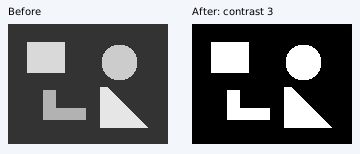
Compare linear exposure with encoded grey-value adjustments using synthetic images, histograms and gradients.
Run in your browser
Explore conditions & results →LAB / EXPERIMENT & VERIFY
Change a condition. Compare the results. Verify with code. Make the technology your own, one experiment at a time.
Pick a topic and open it in your browser.
Adjust inputs or control settings.
Use plots and numbers to understand why.
Compare linear exposure with encoded grey-value adjustments using synthetic images, histograms and gradients.
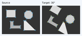
Rotate, resize and change the brightness of synthetic images, then compare detected corners and known reference positions.
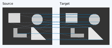
Compare image patches, filter proposed correspondences and see why geometric agreement does not guarantee a correct match.
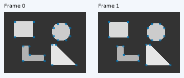
Estimate sparse image motion and compare it with known synthetic motion. Explore brightness changes, occlusion and the aperture problem.
Change the horizon, weights and steering limit, and compare predicted paths, solver convergence and failure handling in your browser.
Run five trackers together on one vehicle, path, initial state and steering limit, and compare cross-track error, smoothness and completion with shared metric definitions.
Compare speed-scaled lookahead with PP, including acceleration and minimum/maximum bounds.
Change fixed lookahead and inspect tracking error, steering and targets on a shared vehicle model.
Separate lookahead from speed regulation and compare curvature limits, speed floors, final approach and actual vehicle speed.
Separate front and rear axle errors and compare gain, speed and steering constraints in your browser.
Combine CO₂, EC, pH, DO, flow, level and pressure to separate spatial differences, instrument bias and sample transport delay. Check circulation, ventilation and water-balance residuals.
Integrate a synthetic one-zone model in Python and verify how LED heat, outdoor exchange, ventilation, capacitance and cooling change room temperature.
Treat room temperature and vapour mass as two states, then define interactions and test conditions for cooling, dehumidification, reheat and ventilation.
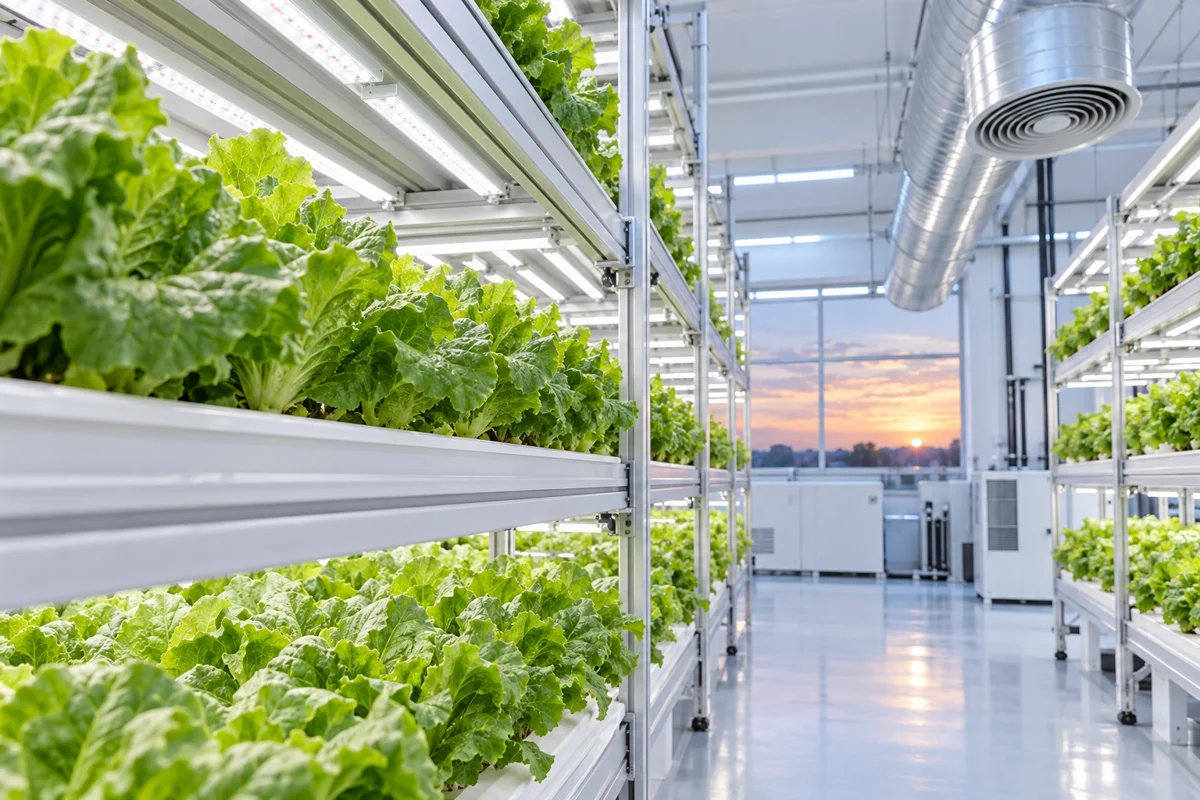
Connect photosynthesis, respiration, stomata, and water transport to environmental measurements. Two synthetic calculations separate carbon gain from harvest mass and vapor pressure deficit from transpiration.
Calculate air VPD and daily light integral from synthetic CSV, testing unequal intervals, missing data and unit mistakes.
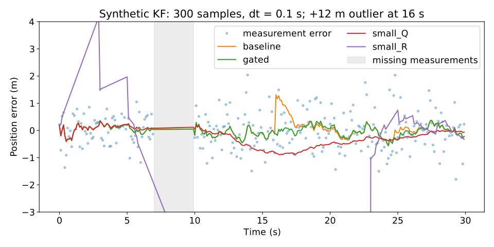
Compare Q, R and outlier gating on one synthetic trajectory using estimation error and rejected observations.
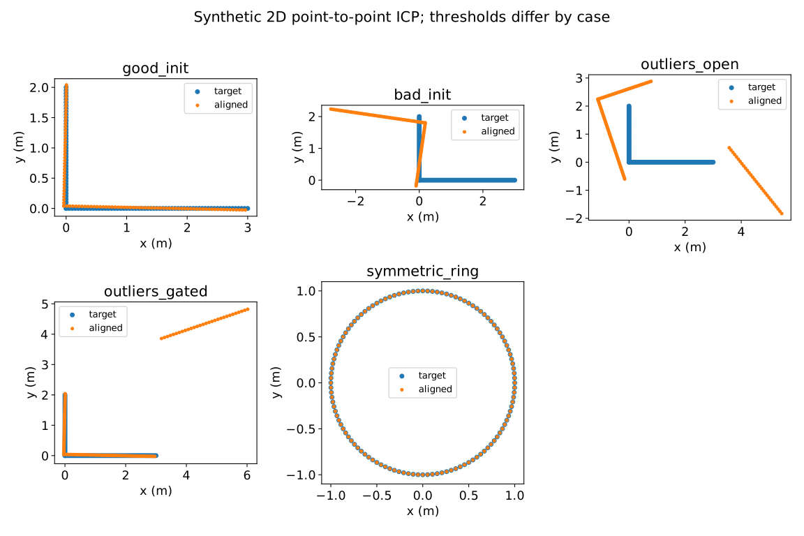
Run 2D registration and distinguish residuals, correspondence coverage and true pose error.
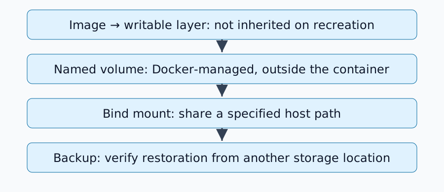
Distinguish writable layers, named volumes and bind mounts, then verify persistence across container recreation.
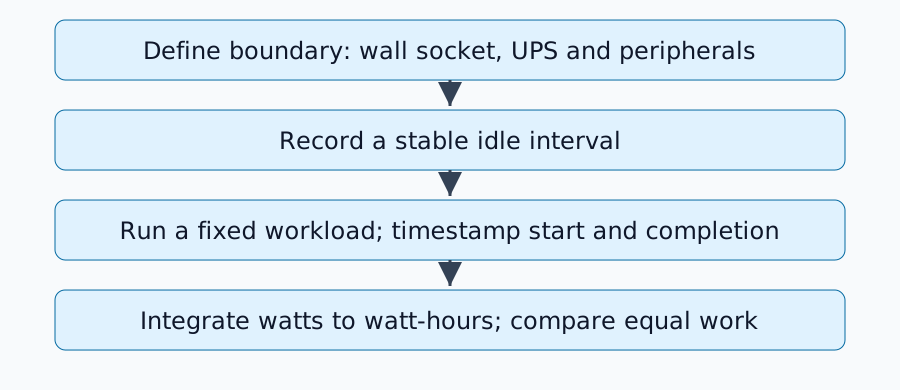
Log wall-side active power consistently and compare idle demand and energy per completed workload.
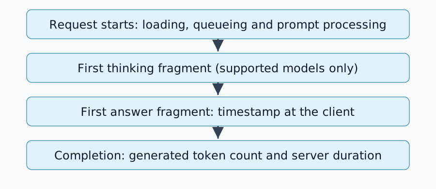
Measure first answer content separately from generation rate and control residency, caching and memory conditions.
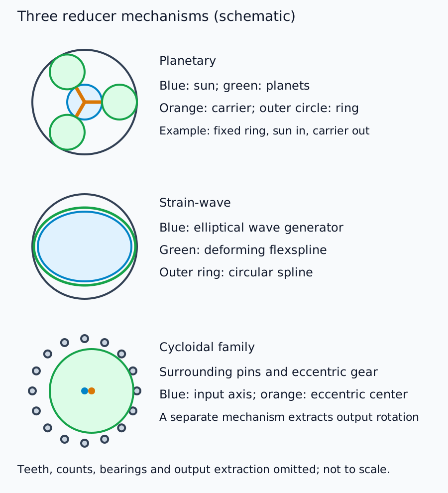
Compare three mechanisms and connect speed, torque and inertia with selection criteria beyond backlash.
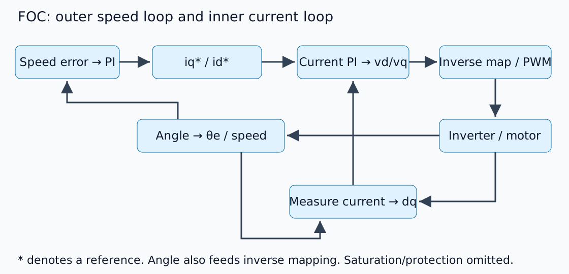
Understand how speed control requests current and how FOC connects rotating coordinates, electrical angle and limits.
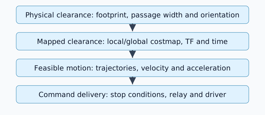
Inspect geometry, costmaps, control feasibility and command delivery to explain a stopped robot.
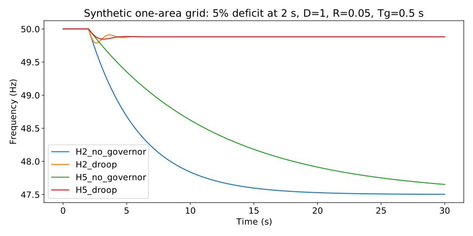
Use a simple one-area model to separate inertia from primary frequency response after a supply deficit.
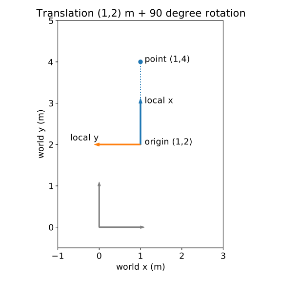
Use a numeric example to connect rotation, translation, inverse transforms, quaternions and ROS frames.
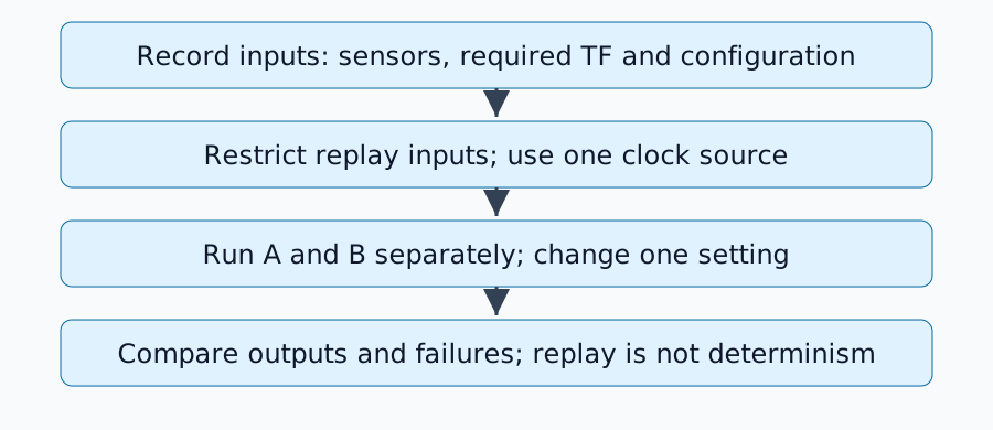
Build controlled replay comparisons and diagnose duplicate TF publishers and mixed time sources.
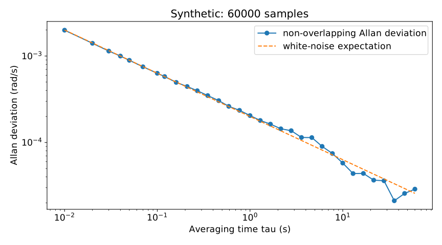
Compute mean, standard deviation and non-overlapping Allan deviation without overinterpreting a short gyro log.
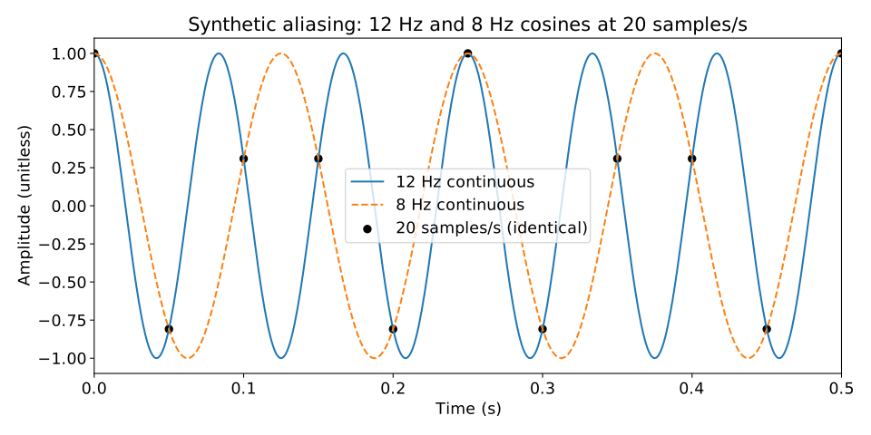
Reproduce identical samples from 12 Hz and 8 Hz signals and distinguish ODR, bandwidth, polling and decimation.
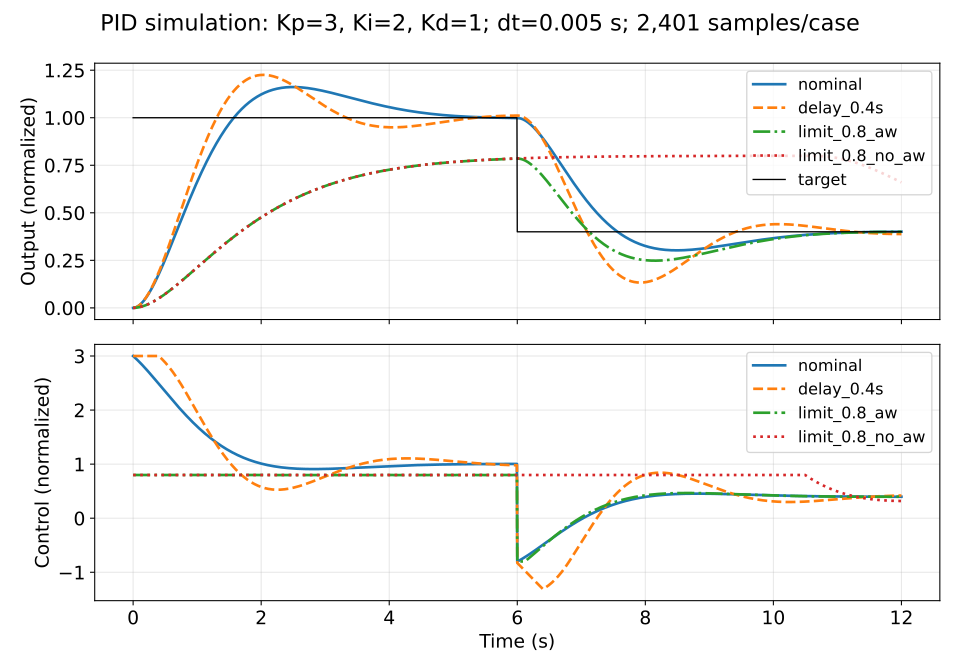
Reproduce how measurement delay, actuator limits and integral windup change PID tracking on the same second-order model.
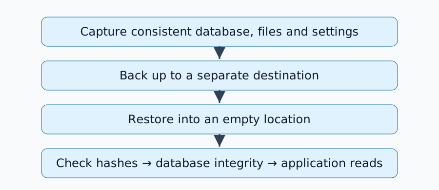
Distinguish restored files from usable application data with a small SQLite exercise, then map the checks to a real server.
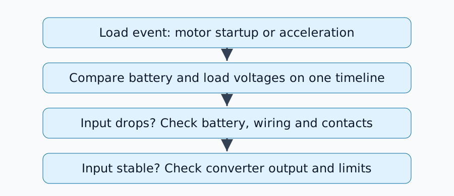
Relate motor load changes to voltage drops and locate faults across the battery, wiring, converter and computer.
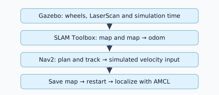
Use the Jazzy simulation to check mapping, map saving, reloading and goal navigation as separate steps.
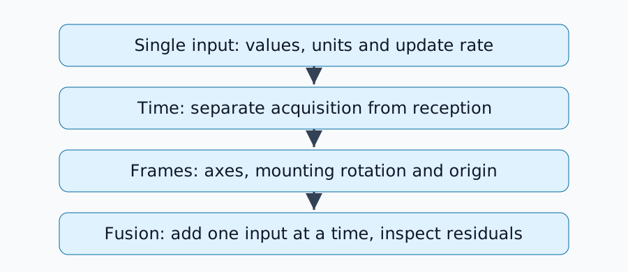
Diagnose fusion failures through timestamps, coordinate frames, mounting geometry and covariance.
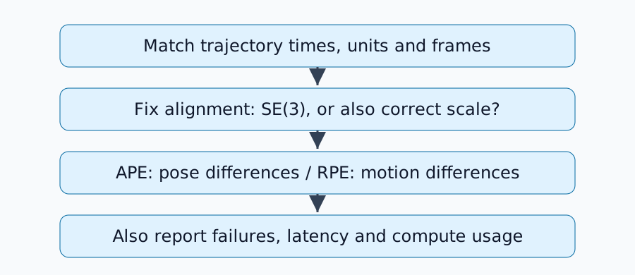
Use synthetic trajectories to distinguish absolute and relative errors, then define matching, alignment and failure reporting for an evaluation.
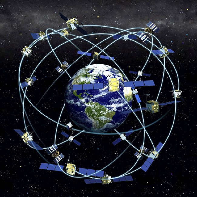
RTK combines satellite positioning with correction data from a base station, shrinking the several-meter error of standalone GNSS positioning down to centimeter level. We work through how dual-frequency positioning cancels ionospheric delay, how u-blox's ZED-F9P drove low-cost RTK into the mainstream, Trimble RTX and Japan's own Michibiki (QZSS), and the real-world example of Kubota's nationwide network of 342 RTK base stations for farm machinery — and how each of these changes what positioning accuracy you actually get.