Read a stationary IMU log: bias, scatter and Allan deviation

A nonzero stationary IMU output is not all random noise. Separate average offset, short-term scatter and stability across averaging times. This article analyzes one gyro axis with a CSV tool validated on synthetic data of known properties.

Establish stationary conditions and valid time

Fix the IMU and record warm-up, output rate, filtering, temperature, duration and units. Desk vibration, cable forces or changing temperature invalidate a sensor-noise-only interpretation. Stationary accelerometers include gravity, so do not transfer the gyro's near-zero expectation to acceleration.

Mean angular rate may contain more than bias, including Earth rotation when sensitivity and installation make it relevant. The ADI evaluation guide motivates disturbance-free, temperature-controlled recordings; its device-specific acquisition settings are not universal IMU requirements.

CSV and reproduction

Use columns time_s,gyro_rad_s, in seconds and rad/s. Download the analysis script:

python3 imu_noise.py --synthetic
python3 imu_noise.py stationary.csv

The second line is an alternative invocation for your own file. Synthetic mode was executed with Python 3.12.3, NumPy 1.26.4 and Matplotlib 3.6.3. Inputs need at least 100 finite samples, strictly increasing times and interval deviations no greater than 1% of the median interval. That 1% is this exercise's validation rule, not an IMU specification.

Do not close gaps and pretend sampling was uniform. Split continuous intervals first. Resampling also changes noise through interpolation/filtering and should be documented.

Mean and standard deviation

Synthetic inputs contain 60,000 points over 600 s at 100 Hz, seed 7: a constant 0.01 rad/s offset plus independent Gaussian noise with 0.002 rad/s standard deviation. Results are mean 0.009991 rad/s and sample standard deviation 0.001994 rad/s. Download the input and statistics.

The mean characterizes this interval, not every temperature or power cycle. Standard deviation alone does not adequately separate slow changes from fast noise. Vary the averaging time next.

Allan deviation across averaging times

Split angular rates into K non-overlapping blocks of m samples, with block means ȳ. The implemented statistic is:

Units remain rad/s. For each m, trailing samples that cannot form a complete block are discarded. Differencing adjacent means cancels a constant offset, so Allan deviation alone cannot reveal its magnitude. NIST SP 1065 explains the definition and overlapping variant. Although that reference concerns frequency stability, this code applies the adjacent-mean statistic to gyro angular rates.

Read the synthetic result

Diagram 1 · Use the button to switch views

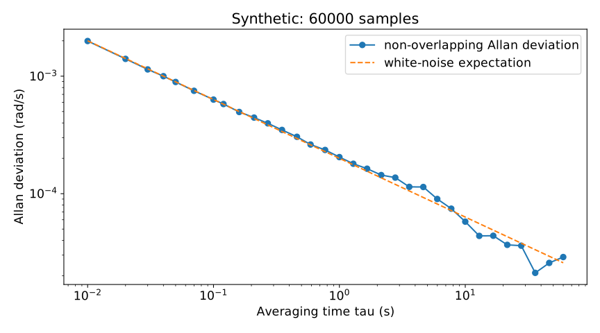
For independent white noise, averaging m samples reduces scatter approximately as 1/√m. The plotted theoretical curve is 0.002/√(100τ). Long averaging times have fewer blocks and more uncertain estimates. The Allan CSV includes adjacent_pairs. At least ten blocks are required, but roughly nine adjacent pairs at the end still provide weak evidence.

No bias instability or random walk was added. A falling curve says nothing about long-term stability of a real IMU. Identifying its minimum as bias instability also requires checking the noise model, slope and convention-dependent coefficient.

Record enough conditions to compare

Save model/firmware, ODR, bandwidth, units, temperature range, total duration, missing-data rate, axis, mean, standard deviation and pair counts for each τ. ODR is the sensor's internal output data rate, not host polling frequency. Filtering changes curves even on identical hardware. Continue with sampling and aliasing to understand why faster polling alone creates no new information.