Sampling and aliasing: why faster polling is not enough

Polling a sensor faster may only retrieve the same value repeatedly. A low-frequency feature in sampled data may also be a folded high-frequency input. This experiment shows two different continuous signals producing indistinguishable samples.

Separate four rates and bandwidths

ODR is the rate of new sensor output; polling is how often the host reads it. Bandwidth describes which input frequencies pass, while logging rate describes what is retained. A 100 Hz ODR does not specify bandwidth independently of internal filtering. Polling the same register at 1 kHz need not yield 1,000 fresh samples.

With FIFO devices, batch arrival time also differs from individual acquisition times. Check device timestamps rather than treating arrivals as uniformly timed measurements.

Two waves, identical samples

At a 20 Hz sample rate, timestamps are n/20 s. These 12 Hz and 8 Hz cosines coincide:

Because 12=20−8, removing the integer-cycle phase leaves a sign reversal. Cosine is even, yielding the equality. This is a phase-aligned cosine example, not a claim that arbitrary signals retain identical appearance.

Run and inspect

Download the script and run python3 engineering_labs.py. It was executed with Python 3.12.3, NumPy 1.26.4 and Matplotlib 3.6.3. Across 40 samples from 0 through 1.95 s, maximum difference is approximately 2.24×10⁻¹⁴, consistent with floating-point rounding. Inspect the CSV in a spreadsheet too.

Diagram 1 · Use the button to switch views

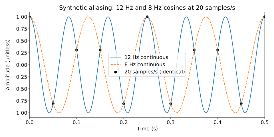
The figure zooms to 0–0.5 s. Continuous curves differ but black samples coincide. These samples alone cannot identify which input produced them.

Nyquist conditions have assumptions

For baseband reconstruction, keep the highest input frequency comfortably below half the sampling rate. Near equality, phase can even produce all-zero samples, so exactly twice the frequency is not a practical margin. Out-of-band vibration and noise fold too. See the ADI antialiasing explanation.

Once unwanted content has folded into the signal band, later smoothing alone cannot separate it from the original signal. The ADC aliasing explanation distinguishes pre-sampling analog filtering from subsequent processing.

Decimation can introduce another alias

Keeping every fifth sample of a 100 Hz log yields 20 Hz. A correctly recorded 12 Hz component now exceeds the new 10 Hz Nyquist frequency. Low-pass filter for the new bandwidth before downsampling, accounting for transition band and delay.

Averaging changes frequency response but does not guarantee sufficient out-of-band rejection. A smooth graph and successful antialiasing are separate claims.

Check real logs in order

Inspect ODR, internal filters, FIFO and timestamp meaning. Use counters and intervals to find duplicates and gaps. Compare multiple rates with known inputs or stable conditions. A spectral peak that moves when the rate changes suggests aliasing, but mechanical operating conditions must also stay fixed. Complete these checks before interpreting IMU noise statistics.