Contents — find the section you need
Background and reading guide
Background Units used in specifications, such as voltage, current, distance and time.
Fundamentals · Explanations of principles, structure and trade-offs.
A rotary encoder is a sensor that converts a rotating shaft's angle or rotational speed into an electrical signal, used for measuring motor rotation rate and for wheel odometry (estimating distance traveled and pose from wheel rotation). The underlying principle splits broadly into two: optical, which reads a disc alternating between transparent and opaque segments with light, and magnetic, which reads the direction of a magnetic field generated by a magnet using a Hall-effect element — these are the two dominant currents in rotary encoders today.
Principle: converting rotation into electrical pulses
Most incremental encoders output two signals, phase A and phase B, offset by 90 degrees. A single signal alone can count rotations (pulses) but can't determine direction; with two signals offset in phase, direction can be determined by which phase leads. This scheme is called a quadrature signal.
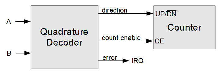 Quadrature decoder circuit
Image: QuadratureDecoder (Lambtron, CC BY-SA 4.0), Wikimedia Commons.

The number of pulses per revolution (PPR, or CPR for Cycle Per Revolution) sets the encoder's intrinsic resolution, but where "1x decoding" counts only the rising edge of phase A, "4x decoding" counts all four edges — phase A rising and falling, plus phase B rising and falling — multiplying the effective resolution by 4 on the same physical disc. The effective count obtained per revolution, N_{count}, can be written as:
Here k_{quad} is the multiplication factor (1, 2, or 4). From this effective count and the diameter D of the wheel (or gear), the distance traveled per count d can be derived.
Most magnetic encoders determine angle through a different principle from this pulse-counting scheme. When the magnetic field of a 2-pole magnet mounted on the shaft is sensed by two Hall-effect elements placed 90 degrees apart, the result is a sine-wave and a cosine-wave signal, V_{\sin} \propto \sin\phi and V_{\cos} \propto \cos\phi, as a function of rotation angle \phi. Taking the arctangent of these two signals yields the angle itself directly and continuously, rather than counting pulses.
This scheme goes through internal A/D conversion and digital signal processing (arctangent computation via a CORDIC algorithm, for instance) before emerging as a digital output such as SPI or PWM. The very concept of a missed pulse doesn't exist here, but in exchange, nonlinearity inherent in the magnetic field itself and eccentricity in the magnet's mounting (a center offset) become error sources.
Another important distinction is between incremental and absolute types. An incremental encoder outputs only relative change, treating whatever position it's at right after power-on as the "origin," whereas an absolute encoder can recover the shaft's absolute angle the instant power is restored, even after being switched off. Gray code (reflected binary code) is often used in absolute-encoder implementations, designed so that adjacent values always differ by exactly one bit. In ordinary binary, transitioning from 3 (011) to 4 (100), for example, requires three bits to switch simultaneously, and even a slight misalignment in read timing risks misreading an entirely different value (111 or 000, say). Because Gray code changes only one bit at a time, this kind of misread can't happen in principle, and it's widely used as the encoding scheme for absolute encoders that read absolute angle directly from multiple optical or magnetic tracks.
Optical vs. magnetic: a tradeoff between precision and robustness
Optical encoders rotate a glass or plastic disc, alternately patterned with transparent and opaque segments, between a light source (typically an LED) and a photodiode, converting the transmission or blocking of light into an electrical signal. By dividing the tracks finely and combining multiple sensors, current products can achieve the highest class of resolution and precision available. The catch is vulnerability to dust, moisture, and oil that physically block the light path, and a need for precise alignment, which together pose a challenge for robustness in harsh environments.
Ultra-high-precision products like the Renishaw RESOLUTE push this subdivision even further, achieving a resolution of 1nm in linear terms and holding sub-divisional error (SDE — the error arising from electrically interpolating optical interference fringes) to within ±40nm. In exchange, the slightest contamination, condensation, or oil film on the light path changes the transmitted light intensity, directly causing read errors or dropped pulses — which tends to make a sealed housing and periodic cleaning practical prerequisites for operation.
Magnetic encoders detect the magnetic field generated by a small permanent magnet mounted on the shaft using an IC with a built-in Hall-effect element, and compute angle from the field's direction. Because of nonlinearity inherent in the magnetic field itself, magnetic encoders have historically been considered less capable of the resolution and positional accuracy optical encoders reach — though products like the AS5048A, discussed below, have arrived at a practical resolution of 14 bits (16,384 divisions). Their biggest strength is robustness: needing no light path, they can operate in humid, dusty, or vibration-heavy environments, or even ones exposed to liquid. Requiring no additional driving element like an LED light source also tends to give them an edge in power consumption and parts count. On the other hand, "eccentricity" — the magnet's mounting position sitting slightly off the rotation center — is known to show up as a low-order harmonic component in angular error, and the more precise a magnetic product aims to be, the more it matters to implement software-side compensation algorithms for this eccentricity error (harmonic decoupling via a phase-locked loop, for instance). Research improving eccentricity-compensation algorithms was published in a Chinese academic journal as recently as 2026, underscoring that improving magnetic-encoder accuracy remains an active research area.
Key product specification comparison
| Product | Type | Resolution | Output | Voltage | Notes |
|---|---|---|---|---|---|
| Broadcom HEDS-9040 | Optical, incremental | 1000–2000 CPR (3-channel, with index) | Quadrature + index | 5V | Up to 30,000rpm, -40 to 100°C; widely proven in DC motor applications |
| US Digital E4T | Optical, incremental (compact) | Up to 4096 CPR (before quadrature) | Quadrature + index, single-ended or differential | — | Compact design fits motors as small as NEMA size 8 |
| Renishaw RESOLUTE | Optical, absolute (ultra-precision) | 1nm (linear), total installed accuracy ±1 arc-second (rotary) | Serial (absolute value, position acquired instantly on start-up) | — | Up to 36,000rpm, SDE (sub-divisional error) ±40nm |
| ams OSRAM AS5048A | Magnetic, absolute | 14-bit (16,384 divisions, 0.0219°/LSB) | SPI/PWM | 3.3–5V | Contactless (2-pole magnet on-axis), accuracy 0.05° after linearization |
| CUI (Same Sky) AMT102-V | Magnetic, incremental | 48–2048 PPR (DIP-switch selectable, up to 8192 counts/rev with 4x quadrature) | Quadrature + index | 5V | Modular kit supporting 288 shaft/mount configurations |
Comparing the three optical products shows how differently "optical" can play out depending on application. The Broadcom HEDS-9040 is a general-purpose part with a long track record as DC motor feedback, while the US Digital E4T pursues a compact, lightweight design that mounts even on a NEMA size 8 motor. The Renishaw RESOLUTE serves an ultra-precision use case (machine-tool positioning, for example) that's literally an order of magnitude beyond either of those two. The two magnetic products, the AS5048A and AMT102-V, adopt different output schemes — absolute and incremental, respectively — sharing the convenience of contactless on-axis mounting while splitting on whether an absolute position is needed or a relative rotation amount suffices.
Looking purely at digit count of resolution, the AS5048A's 14 bits (16,384 divisions) appears to beat the HEDS-9040's 2000 CPR (equivalent to 8000 counts with 4x quadrature), but the two rest on different measurement principles and can't be compared directly. The HEDS-9040 is a discrete measurement whose resolution is fixed by a physical pulse count, while the AS5048A digitizes a continuous magnetic-field direction through A/D conversion, so its effective angular accuracy also depends on internal noise, magnet quality, and mounting precision. That's exactly why the datasheet's "accuracy 0.05° after linearization" figure comes out coarser than the raw resolution (0.0219°/LSB) — catalog resolution and the angular accuracy actually achieved in practice need to be treated as two different things.
History: a technology born from reproducing pipe organ tones
Baldwin: an organ maker starts optical encoding — The origin of the optical encoder traces back to Baldwin, a piano and organ maker founded in Cincinnati, Ohio, in the 19th century. After World War II, Baldwin pushed to bring electronics into keyboard instruments, engraving transparent and opaque patterns onto glass discs to develop optical encoding technology that electronically reproduced the tones of a church pipe organ. This technology caught the attention of the U.S. Army Signal Corps, which in 1951 contracted with Baldwin to apply this optical disc technology to radar antenna tracking. The company completed its first experimental optical encoder in 1955, deployed an 18-bit encoder for space use in 1962, and by 1963 had the first optical encoder with an LED light source flying in space. A technology an instrument maker happened to invent went on to bloom in fields — military and space technology — utterly unrelated to its origin. Around the same time, Germany's Heidenhain company independently established its own "diadur" process for forming precise chromium structures on glass in 1950, produced optical length-measuring devices for machine tools by 1952, and completed its first photoelectric incremental rotary encoder in 1961 — meaning the practical development of optical encoders proceeded in parallel in both the US and Germany.
The founding of US Digital, whose product appears in the comparison table above, is itself another example of the "I was stuck, so I built it myself" origin story so common in this industry. In 1980, an engineer named David Madore, working at a medical ultrasound equipment company, ran into a problem: the optical encoders his company's product needed were too expensive on the market at the time, had long lead times, and weren't available with the specs he actually wanted. So Madore manufactured his own first encoder to fill the gap — and that became the origin of US Digital itself. It's necessity-is-the-mother-of-invention playing out literally, and following Baldwin and Heidenhain, it suggests a pattern that's repeated in this field: an engineer driven by need becomes a new supplier in their own right.
Frank Gray: a code invented for error correction becomes the encoder standard — Frank Gray, the inventor of the eponymous Gray code, was a researcher at Bell Labs. He filed a patent for the scheme in 1947, granted in 1953, aimed at minimizing errors (misreading an adjacent value) that arose in the process of digitizing analog signals via pulse code modulation (PCM). It was originally devised for error correction in communications technology, but the property itself — "adjacent values differ by only one bit" — turned out to be ideal as an encoding scheme for absolute encoders that read multiple tracks at once, and the technique got repurposed into the rotary-encoder field years later. It's a fine example of a code invented for one purpose becoming, decades later, a standard technology in an entirely different field.
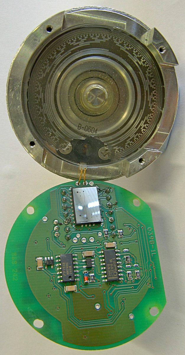 13-track Gray code absolute encoder
Image: Gray code rotary encoder 13-track opened (Mike1024, public domain), Wikimedia Commons. The top shows the housing, interrupter disk, and light source; the bottom shows the reflective sensing element (marked "OPTOLAB") and support circuitry. This particular encoder was reportedly removed from a machine after water ingress caused the Gray code tracks to lift off.

As the pictured unit shows, arranging multiple tracks concentrically to be read all at once leaves Gray-code absolute encoders somewhat vulnerable to water ingress. Each track carries one bit, so adding more tracks raises resolution (bit count) — but parts count and failure points rise right along with track count, and this photo embodies that precision-versus-robustness tradeoff.
Quadrature decoding and validation
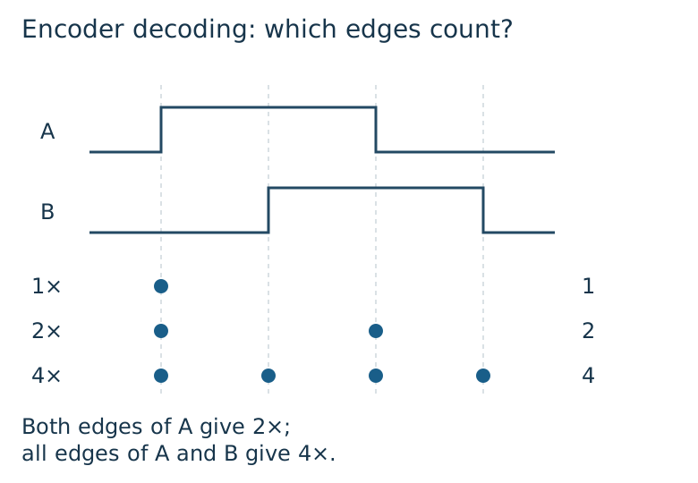
Direction follows the phase relationship between channels A and B. 1× decoding counts one edge of A; 2× counts both edges of A; 4× counts all edges of both A and B. An interrupt on changes of A alone provides 2× decoding, even when B is read to determine direction.
Apply a known number of revolutions and compare the count against the datasheet definition of PPR/CPR and the selected decoding mode. Check missed edges at speed, extra transitions caused by noise, and the sign during reversal separately. A dedicated counter reduces CPU interrupt load, but does not remove signal-quality limits, input-frequency limits, or wheel slip.
Wheel odometry, the downstream application: how does error propagate?
Let d_L and d_R be the left and right wheel travel distances obtained from the encoders, and L the distance between the wheels (tread width). The turning angle \Delta\theta and translation distance \Delta s over a short time interval are then computed as:
Integrating this \Delta\theta and \Delta s into the current pose (x, y, \theta) step by step is the basic algorithm of wheel odometry. The equation also shows that the narrower the tread width L, the more the same count error gets amplified into turning-angle error.
Fusing LiDAR, IMU, and wheel encoders is becoming the default — where the research stands now
A March 2026 paper, "Intelligent Control of Differential Drive Robots Subject to Unmodeled Dynamics with EKF-based State Estimation" (Alwala, Hu, da Silva Lima, Bessa), builds a control framework combining Lyapunov-based nonlinear control with adaptive neural networks, into which it wires an EKF (Extended Kalman Filter) that fuses multiple odometry sources: IMU, monocular camera, 2D LiDAR, and wheel encoders. What the paper emphasizes is robustness — maintaining consistent performance even under drift, wheel slip, sensor noise, and sensor failure — reporting an improvement of up to 53.91% in linear velocity error versus a baseline (feedback linearization control). What this corner of the research field is showing is that "raise the encoder's resolution and noise immunity" (a hardware-side improvement) and "cancel error out across multiple sensors" (a software-side improvement) aren't competing options — they're two wheels of the same cart, meant to be used together.
What makes this paper interesting is that it keeps the wheel encoder in the EKF as an information source on equal footing with the others, rather than treating it as a sensor to discard. It's a design that automatically lowers the encoder's weight only at the moment wheel slip or failure occurs, while otherwise leaning on wheel odometry's real strength — accurately capturing short-term relative displacement without the expensive feature-matching that LiDAR or camera-based methods require, updating with lightweight computation on every sampling cycle.
Parameters that determine performance
- Resolution (PPR/CPR) and multiplication: Switching from 1x to 4x decoding on the exact same physical disc quadruples effective count resolution. Finer increments do not by themselves imply better absolute accuracy.
- Environmental tolerance: In outdoor, dusty, or vibration-heavy environments, a magnetic encoder that needs no light path tends to have the edge. In a controlled environment like a cleanroom or a machine tool, optical's higher resolution and precision can be put to full use
- Absolute vs. relative: An incremental encoder needs a homing operation to re-establish its origin every time power cycles, while whether an absolute encoder like the AS5048A can recover instantly from a power loss directly affects how complex the whole system's startup sequence needs to be
- Tread width and error amplification: From \Delta\theta = (d_R - d_L)/L, the narrower the vehicle's left/right wheel spacing, the more the same encoder count error gets amplified into turning-angle error. Smaller robots face relatively stricter demands on encoder resolution and reliability
- Single-sensor accuracy vs. multi-sensor fusion: As the 2026 EKF research shows, pushing an encoder's own accuracy through hardware and fusing it with IMU/LiDAR/etc. to cancel error through software aren't an either/or choice — robustness only comes from combining both
- Sampling frequency and timing precision: In applications with high-speed rotation or abrupt speed changes, dropped pulses or interrupt-timing jitter translate directly into miscounts.
- The gap between catalog resolution and effective accuracy: As with the AS5048A's raw resolution of 0.0219°/LSB versus its post-linearization accuracy of only 0.05°, datasheet resolution and the angular accuracy a system actually achieves are two different things. Comparing products purely on digit count of resolution risks overestimating the accuracy you'll get in practice
- Decoder validation: Check the count over a known number of revolutions and verify the sign during reversal
- Tolerance to eccentricity/alignment error: In magnetic encoders, mounting eccentricity of the magnet shows up as low-order harmonic angular error; in optical encoders, even a slight misalignment between disc and light source/photodetector translates directly into read error. In either scheme, mounting precision — not just the sensor's own spec — determines final performance
- Power consumption and parts count: Requiring an LED light source and a photodiode, optical encoders tend to lose out to magnetic ones on parts count and power draw. For a battery-powered small robot, this gap can be the deciding factor in product selection
- Cost and availability: An ultra-precision product like the Renishaw RESOLUTE sits in a high price bracket aimed at machine tools and industrial robots, while a capacitive product like the AMT102-V — switchable between 48 and 2048 PPR with a single DIP switch — cuts prototyping-stage cost and tuning effort substantially. For an individually developed robot project, this gap in availability and price bracket becomes a real practical constraint on hardware selection
Does higher encoder resolution guarantee greater absolute accuracy?
Eccentricity and scale errors are separate from resolution. Distinguish increment size, repeatability, and absolute accuracy.
References
- HEDS-9040/9140 datasheet (Broadcom)
- E4T Miniature Motor Encoder datasheet (US Digital)
- RESOLUTE absolute optical encoder system data sheet (Renishaw)
- AS5048A/AS5048B datasheet (ams OSRAM)
- AMT102-V datasheet (CUI Devices/Same Sky)
- A Comparison of Encoder Technologies (Oriental Motor)
- Magnetic vs Optical Encoder (POSITAL)
- Absolute vs. Incremental Rotary Encoders (Design News)
- How Encoder Tech Evolved Over Time (US Digital)
- Gray code (Wikipedia, references Frank Gray's 1947 filing / 1953 patent grant)
- Gray Code Rotary Encoder (Quantum Devices)
- Error Suppression of Magnetic Encoder Using Improved Harmonic Decoupling (Chinese Journal of Electrical Engineering, 2026)
- Same Sky — AMT102-V
Current step · 9 / 21 · Sensors & Hardware
Comments
Please log in to post a comment
No comments yet.