Run a Kalman filter in Python: noise, missing data and outliers

Kalman tuning expresses uncertainty in a motion model and its observations. This experiment estimates position and velocity, then compares prediction during missing data, reactions to an outlier and rejection caused by overconfidence. All inputs are synthetic; the numbers are not hardware accuracy claims.

Model and units

The state contains position [m] and velocity [m/s]. Only position is observed, every 0.1 s:

Observation standard deviation is 0.7 m, giving R=0.49 m². Process covariance is q ggᵀ with g=(dt²/2, dt), representing an independent acceleration perturbation per step. Here q=0.4 has units (m/s²)²; it is not a continuous white-noise spectral density. Do not transfer this value to another discretization without checking its meaning. See the Kalman filter introduction for prediction and update derivations.

For the theory, see Simo Särkkä (2013), Bayesian Filtering and Smoothing, section 4.3. Trajectory, gate and comparison conditions here are our own experiment design.

Four configurations, identical input

Save the experiment script in an empty output directory and run:

python3 engineering_labs.py

Execution was checked with Python 3.12.3, NumPy 1.26.4 and Matplotlib 3.6.3. The file also produces the other linked engineering experiments. It uses seed 42 and 300 samples. True velocity changes from 1 to 1.4 m/s at 12 s. Thirty observations from 7.0 through 9.9 s are missing, and 12 m is added to the observation at 16 s. Initial position/velocity are 0 m and 1 m/s; initial covariance has diagonal entries 1 m² and 1 (m/s)². Each configuration receives exactly the same observations.

Normalize the residual

Let e be the observation residual before correction and S its predicted variance. The gate rejects an observation when:

This threshold applies to this scalar normalized residual, not arbitrarily to multidimensional observations. Missing or rejected measurements trigger prediction without correction. The implementation uses the Joseph covariance update and checks positive semidefiniteness. Uncertainty grows during missing data, so this differs from a fixed rejection distance in metres.

Results reveal overconfidence

Diagram 1 · Use the button to switch views

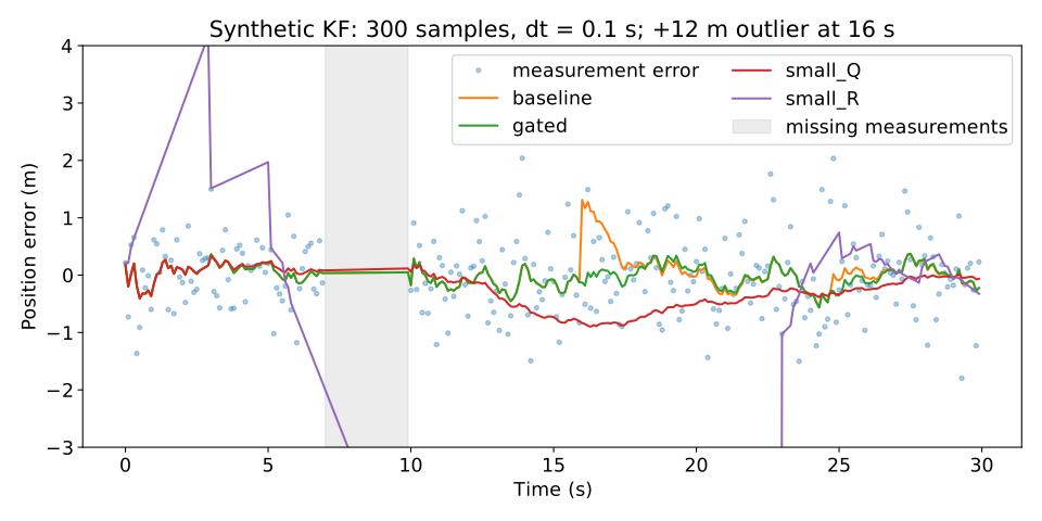
The vertical range is limited to −3 through 4 m for comparison. The 12 m outlier and large errors with small R extend beyond it. Inspect the gated CSV, small-R CSV and complete summary for uncropped values. CSV missing observations are nan and do not count as rejections.

The gate rejects two observations, although only one artificial outlier was injected. A threshold does not identify only deliberately corrupted samples. Underestimating observation variance by a factor of 100 causes 237 rejections: normal scatter becomes incompatible with the filter's confidence. Lost corrections then prevent tracking the velocity change, making residuals even larger. Adding a gate alone does not create robustness.

Moving to your own logs

Check timestamps, units and frames first. Estimate observation variance on stationary intervals, then examine motion-model errors and residuals during motion. Introduce gating last, reporting missing-data rate, rejection rate and uncertainty along with RMSE. Real hardware needs an independent reference to calculate comparable errors.

Small Q can make a curve smooth while increasing lag. Increasing Q is not universally better either. These rankings apply only to this trajectory, initialization, noise and evaluation window.

Follow-up check

The sigma_m column is estimated position standard deviation. Plot the estimate plus/minus twice sigma and compare the missing-data interval with the velocity change. This separates actual error from the estimator's self-assessment. Continue with sensor-fusion debugging to diagnose timing and TF before changing covariance.

Run the same calculation locally

Extract the complete runnable source ZIP, or save the experiment entrypoint, generated kernels, and original PID source in one folder. PID uses the Python standard library; Kalman and ICP require NumPy. The original figure-generation commands remain available.

python3 -m pip install numpy==1.26.4
python3 experiment.py kalman --parameters '{"q":0.4,"r":0.49,"gate":false}' > result.json

Toggle gate to compare the outlier response, then set q to 0.002 or r to 0.0049 and compare RMSE and rejection count. Observations are fixed from the saved CSV across runs.