Control Engineering Primer: LQR — State Feedback From Explicit Priorities

Contents — find the section you need

Background and reading guide

Background Basic functions, calculus and vectors; follow the definitions alongside the equations.

Fundamentals · Explanations of principles, structure and trade-offs.

Linear Quadratic Regulation (LQR) assigns a cost to state deviation and to using an actuator, then derives the state-feedback law that minimizes that cost for a linear model. Unlike PID, which directly reacts to the present error, its history, and its rate, LQR can use position, velocity, angle, angular rate, current, and coupled axes as one state. It is especially clear for local stabilization of an inverted pendulum, aircraft attitude, balancing robot, or robot arm.

LQR is not a magic optimality switch. If required state is unmeasured, an observer is needed; if the plant leaves the range of a local linear model, the gain loses its promise; and if input or state constraints are central, MPC is often the better layer. For the ROS 2 execution boundary, see ROS 2 Primer; for estimation assumptions, see Sensor Fusion Primer.

Practical conclusion

From $\dot{x}=Ax+Bu$ and weights $Q,R$ , infinite-horizon LQR produces $u=-Kx$ . $Q$ expresses how strongly state error is penalized; $R$ expresses command cost.
The gain $K$ comes from a Riccati equation and its solution $P$ : $K=R^{-1}B^TP$ . It accounts for modeled coupling instead of manually tuning one gain per state.
Stabilizability of $(A,B)$ and detectability/observability of $(A,C)$ are prerequisites. Having a sensor is not the same as being able to reconstruct the required state.
LQR itself does not enforce actuator limits, collision clearance, or emergency stopping. Those belong to limits and safety functions outside the gain.

State space and signal flow

A state $x$ is the smallest collection of variables which, together with input and disturbance, determines future behavior. A cart needs position and velocity; a rotating body needs angle and angular velocity; an electromechanical drive may add current. A linear time-invariant model is

\dot{x}=Ax+Bu+Ew,\qquad y=Cx+Du+v

where $u$ is command, $w$ unmodeled disturbance, $y$ measurement, and $v$ sensor noise. $A$ describes state evolution, $B$ the input path, and $C$ what sensors reveal.

In the diagram, the summing junction forms $e=\hat{x}-x_r$ (estimated state minus reference), and LQR outputs $u=-Ke$ . For a zero reference this reduces to the usual $u=-K\hat{x}$ .

Diagram: Duskcoil, conceptual rather than measured. A real implementation also has calibration, timestamps, transport delay, and actuator inner loops.

Around an equilibrium $(x_e,u_e)$ , define deviations $\tilde{x}=x-x_e$ and $\tilde{u}=u-u_e$ , then design on $\dot{\tilde{x}}=A\tilde{x}+B\tilde{u}$ . This is a local statement. A gain stabilizing an upright pendulum near zero angle is not necessarily a recovery controller for a pendulum that has fallen far away or a system whose actuator is saturated.

Riccati equation and cost

Continuous infinite-horizon LQR minimizes

J=\int_0^\infty\left(x^TQx+u^TRu\right)dt

with $Q\succeq0$ and $R\succ0$ . Larger $Q$ makes state error expensive; larger $R$ makes effort expensive. Do not add metres, radians, metres per second, and amperes without scaling. A useful start is diagonal weights based on allowable values $x_{max}$ and $u_{max}$ , such as $1/x_{max}^2$ and $1/u_{max}^2$ .

The continuous algebraic Riccati equation is

A^TP+PA-PBR^{-1}B^TP+Q=0

and its stabilizing solution $P$ gives

K=R^{-1}B^TP,\qquad u=-Kx

This gives the feedback gain $K$ used by the controller.

Sampled systems need a discretized model and a discrete Riccati equation. Continuous finite-horizon problems use a differential Riccati equation; discrete finite-horizon problems use a difference equation; discrete infinite-horizon problems use the DARE. The continuous model matrices are $A,B$ , and the discrete model is $x_{k+1}=A_dx_k+B_du_k$ . Applying a continuous gain as if it were a discrete controller, mixing degrees with radians, or ignoring latency can turn an otherwise correct calculation into an unstable device.

Controllability and observability: check conditions before the gain

The controllability matrix is

\mathcal{C}=[B\ AB\ A^2B\ \cdots\ A^{n-1}B]

For an $n$ -state system, the full-rank condition is $\operatorname{rank}\mathcal{C}=n$ .

Full rank means every mode is controllable; LQR requires $(A,B)$ to be stabilizable and $(Q^{1/2},A)$ to be detectable for the standard stabilizing solution. This is distinct from observability of the sensor pair $(C,A)$ . The observability matrix is

\mathcal{O}=\begin{bmatrix}C\\CA\\\vdots\\CA^{n-1}\end{bmatrix}

Full rank means the state can be reconstructed from output history. See Kalman Filter Primer for the estimator that is normally paired with LQR.

Numerical example: stabilizing a double integrator

For a normalized double integrator with $x=[p\ v]^T$ and acceleration command $u$ ,

A=\begin{bmatrix}0&1\\0&0\end{bmatrix},\quad B=\begin{bmatrix}0\\1\end{bmatrix}

Using $Q=\operatorname{diag}(q_p,q_v)$ gives $u=-k_pp-k_vv$ . It resembles PD, but both gains are selected jointly from model and $Q,R$ . Making $q_p$ large while $q_v$ is tiny invites sharp acceleration and braking; making $R$ too small says actuator use is nearly free. The resulting gain is $K=[k_p\ k_v]$ , with $k_p,k_v$ selected together. Physical bounds $|u|\le u_{max}$ and $|\Delta u|\le r_{max}$ are still necessary. If clipping is frequent, reference shaping, redesign, or constrained MPC is more honest than calling the clipped result unconstrained LQR.

For the continuous double integrator with $Q=I$ and $R=1$ , the same derivation gives $K=[1\ \sqrt{3}]\simeq[1\ 1.732]$ . This is a normalized example, not a gain to copy into hardware: recompute it with the sampled model, mass, actuator limits, and delay of the real system.

Choosing among PID, LQR, and MPC

Method	Strong fit	Inputs	Constraint handling	Main caution
PID	fast single-loop regulation	error/history/rate	external limiter	windup and noise
LQR	local linear multistate stabilization	estimated state	not explicit by itself	model range and saturation
MPC	multivariable prediction with limits	state, model, reference	explicit optimization constraints	deadline and feasibility

Nested designs are common: PID current/velocity loops, LQR local attitude or position stabilization, and MPC for trajectory or constraints. For tracking rather than fixed regulation, use a time-varying reference, feedforward, gain scheduling, or LTV-LQR.

Robot implementation and safety

Encoders, IMUs, cameras, and LiDAR publish at different rates and delays. Do not pass arrival-ordered messages directly as a state. Pass a timestamp-aligned estimate, confidence/covariance, and validity status. ROS 2 lifecycle and hardware interfaces described in ROS 2 Primer are design boundaries, not just software organization.

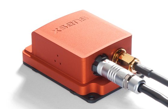Representative IMU/INS

Image: Xsens MTi-G (Kallap85, CC BY-SA 4.0), Wikimedia Commons. It is a representative sensor image, not a measured LQR system or product recommendation.

Monitor estimator covariance growth, sensor timeout, inconsistency between encoder and IMU, sustained saturation, and deadline overruns. If state is no longer trustworthy, do not keep issuing $-K\hat{x}$ . Select a system-specific transition—ramped velocity to zero, torque disable, mechanical brake, or E-stop—based on inertia, gravity, and human proximity. LQR stability claims assume a correct model, correct state and unsaturated input; independent protections must cover the assumptions outside that proof.

Implementation checklist

Fix equilibrium, units, signs, frames, and discrete period.
Measure model residuals near the linearization point and define an operating envelope.
Numerically check controllability and observability/detectability.
Normalize $Q,R$ from allowable state and command; record every change.
Monitor saturation, rate limits, estimate freshness, and independent stopping outside LQR.
Test delay, friction, payload change and sensor loss at low output before expanding the envelope.

References

Check your understanding

What does a larger input penalty encourage?

It encourages conserving control effort. Check the response trade-off and scale state variables with different units appropriately.