Contents — find the section you need
Background and reading guide
Background Basic frames, velocity and sensor terminology; use the reading guide for background.
Fundamentals · Explanations of principles, structure and trade-offs.
Robots and autonomous vehicles typically carry several sensors at once — camera, LiDAR, IMU, radar, GNSS. Yet none of them, alone, understands the world correctly: a camera struggles with depth, a LiDAR can't tell you color or texture, an IMU's errors pile up over time. Sensor Fusion is the technology that fills each sensor's blind spots with another sensor's strengths, assembling one consistent "world model" out of individually flawed pieces. This article works through both mathematical foundations — probability and optimization — and then the concrete pairings: VIO, LIO, and Camera×LiDAR.
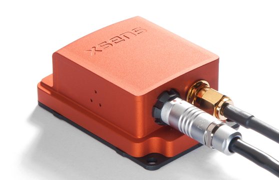 IMU/INS example
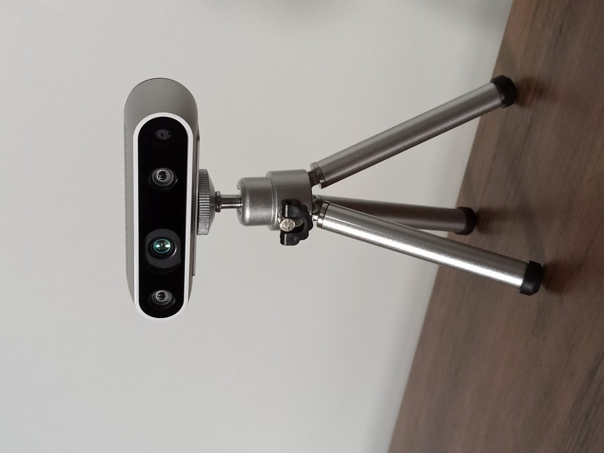 Depth-camera example
Images: Xsens MTi-G (Kallap85, CC BY-SA 4.0) / Intel RealSense depth camera D435 (Marc Auledas, CC BY-SA 4.0), Wikimedia Commons.


0. What This Article Covers
- What Sensor Fusion is for, and why a single sensor is never enough
- The basic Fusion pipeline (sensor → measurement → feature/state → fusion → estimated state)
- The difference between Early, Mid-level, and Late Fusion
- How probabilistic Fusion works — Kalman Filter, EKF, UKF, Particle Filter
- How optimization-based Fusion works — Factor Graphs, Pose Graphs
- Why VIO (Camera×IMU), LIO (LiDAR×IMU), and Camera×LiDAR are such natural pairings
- A four-sensor integration example (Camera×LiDAR×Radar×IMU) using autonomous driving
- What actually makes Fusion hard in practice — time sync, calibration, noise
- How to think about designing a Fusion system for your use case
1. The Short Answer: What Sensor Fusion Is
In one sentence: Sensor Fusion mathematically combines the incomplete, noisy observations from multiple sensors to produce an estimate of "state" that is more accurate and more reliable than any single sensor could give alone.
That definition packs in three ideas. First, complementarity — different sensors are strong and weak in different places, so combining them lets each cancel out the other's weaknesses. Second, State Estimation — the statistical framework for inferring a quantity you can't observe directly (where am I right now, at what velocity, in what orientation) from quantities you can observe. Third, World Model — the result of integrating each sensor's fragmentary information into a single representation that's consistent both in time and in space. A robot doesn't act on raw sensor data — it acts on this integrated World Model.
2. Why Isn't One Sensor Enough?
Lining up what each sensor is good and bad at makes clear why Fusion is essentially mandatory.
| Sensor | Strengths | Weaknesses |
|---|---|---|
| Camera | Recognizes color, texture, and semantics (object category); high angular resolution | Depth is hard to measure directly; weak in darkness, backlight, or bad weather; scale is undetermined (monocular) |
| LiDAR | Precise, direct measurement of distance and geometry; independent of lighting | No color or texture information; struggles in rain, fog, or dust; point clouds get sparse — and less precise — at range |
| IMU (Inertial Measurement Unit) | High sample rate (hundreds of Hz+); sensitive to orientation change; independent of camera illumination and visibility | Affected by temperature, vibration, and mounting error; errors accumulate through integration (drift); gives no absolute position |
| Radar | Resilient to bad weather (rain, fog, dust); measures relative velocity directly via Doppler | Low angular resolution — coarse sense of object shape; can struggle to distinguish stationary objects |
| GNSS | Gives absolute, global coordinates; errors don't accumulate | Low update rate (typically 1–10 Hz); degrades or drops out indoors, in tunnels, or amid urban high-rises (multipath) |
What this table reveals is that "high-precision sensor" and "universal sensor" are two different things. LiDAR beats a camera on geometric precision but can't tell you color or meaning. GNSS gives absolute position but updates slowly and can't be trusted downtown. An IMU does not depend on illumination or visibility, but it is affected by temperature, vibration, and mounting error; because it derives state through integration, drift is unavoidable over time. Sensor Fusion exploits this complementary relationship mathematically.
3. The Basic Structure of Fusion
The details of a Sensor Fusion pipeline shift depending on what's being fused and at what level (the next section), but the broad shape is the same five stages every time.
Figure 1 — Raw measurements from each sensor are converted into features or partial state, and the Fusion stage integrates them into a single estimated state.
Raw measurements straight off each sensor can't be compared directly — they differ in units, coordinate frames, and update rates. Each sensor stream first gets converted into features (image keypoints, point-cloud edges, and so on) or partial state (velocity, relative pose), and only then is it handed to the Fusion stage. That Fusion stage is where the probabilistic methods (Kalman Filters, etc.) or optimization-based methods (Factor Graphs, etc.) discussed below actually live, and its output is the final estimated state — position, velocity, orientation, and more.
4. Three Levels of Fusion
Fusion splits broadly into three levels, depending on where in the pipeline multiple sensors' information gets combined.
| Level | When fusion happens | Characteristics | Example |
|---|---|---|---|
| Early Fusion | Near raw data | Little information loss, potentially very accurate, but demands strict time sync and coordinate alignment between sensors | Projecting a LiDAR point cloud onto a camera image and combining them into one input |
| Mid-level (Feature) Fusion | At the extracted-feature stage | Doesn't demand sync as strict as raw-data fusion; more flexible to implement | BEV-space methods that combine camera and LiDAR features (the BEV Fusion family) |
| Late Fusion | At each sensor's independent perception/estimation output (e.g. detections) | Each sensor's pipeline stays independent, easy to implement, but information lost earlier can't be recovered later | Ensemble-style approaches that combine camera object detections with LiDAR object detections after the fact |
Which level to choose is a trade-off between accuracy and implementation cost. Early Fusion, in principle, exploits the most information, but millisecond-level timing offsets or millimeter-level mounting errors between sensors degrade the result directly, demanding very tight calibration. Late Fusion has a big practical advantage — each sensor's processing pipeline can be developed and debugged independently — but whatever an individual sensor "missed" can't be recovered no matter how cleverly the results are combined downstream. Mid-level Fusion, especially BEV Fusion in autonomous driving, has become the increasingly popular middle ground between these two extremes.
5. Probabilistic Fusion
The first of two mathematical frameworks for combining multiple sensors' observations is grounded in probability theory. Its foundation is Bayesian Estimation: combine "the estimate carried forward from the previous step" (the prior) with "the new observation" (the likelihood) to update "the current estimate" (the posterior).
The left side is the posterior distribution over state x_t given every observation z_{1:t} from time 1 through t. The right side takes the previous estimate p(x_{t-1}\mid z_{1:t-1}), propagates it forward one step through the motion model p(x_t\mid x_{t-1}) (the integral), and then weights that prediction by the likelihood of the new observation p(z_t\mid x_t) — a "predict, then update" cycle.
The Kalman Filter is what you get when you take that general Bayesian update and assume everything — state and observation alike — is linear and Gaussian, which turns the update into a closed-form expression. In the prediction step, the state and error covariance are advanced through the motion model; in the update step, the mismatch between the new observation and the prediction (the innovation) corrects the state, weighted by the Kalman Gain.
P_t^{-} is the predicted error covariance, H maps state into observation space, and R is the observation noise covariance. The Kalman Gain K_t is a weight expressing how much to trust "the model's prediction" versus "the new observation": the smaller the observation noise R (a trustworthy sensor), the more the observation is weighted; the smaller the prediction uncertainty P_t^{-} (a confident model), the more the prediction is weighted — the balance adjusts itself automatically.
A real robot's motion and sensor models are almost never linear, so a plain Kalman Filter usually can't be applied directly. The Extended Kalman Filter (EKF) linearizes the nonlinear motion and observation models around the current estimate using Jacobians, then applies the same update equations as the ordinary Kalman Filter. The Unscented Kalman Filter (UKF; Julier & Uhlmann, 1997) skips the Jacobian approximation entirely, instead passing a small set of representative sample points (sigma points) directly through the nonlinear functions and reconstructing the mean and covariance from the results — which can outperform the EKF under strong nonlinearity. The Particle Filter (Gordon, Salmond & Smith, 1993) doesn't restrict the distribution to Gaussian at all; it approximates the probability distribution itself with a large number of particles (samples), which lets it represent multi-modal distributions where several hypotheses coexist — at the cost of needing more particles, and more compute, for higher accuracy.
6. Optimization-based Fusion
Where probabilistic Fusion updates sequentially, one step at a time, the second mathematical framework — optimization-based Fusion — takes a different approach: hold a window of observations, then re-solve for the state that's maximally consistent with all of them at once.
Its flagship formulation is the Factor Graph. The states to estimate (the robot's pose at each timestep, the positions of observed landmarks) become nodes; the constraints between them (what a given sensor observation tells us about how two states must relate) become Factors connecting those nodes, and the whole graph is solved as a nonlinear least-squares problem.
\mathbf{x} is the full set of states to estimate, \mathbf{z}_k the k-th sensor observation, \mathbf{e}_k the error function measuring the mismatch between what that observation predicts and the current state, and \Sigma_k^{-1} the weight from that observation's confidence. When landmark 3D positions are optimized alongside camera poses, this process is specifically called Bundle Adjustment. When the nodes are poses along a robot's trajectory, it's called Pose Graph optimization — the standard framework for correcting accumulated drift after a loop closure (recognizing a previously visited place).
Probabilistic Fusion (especially the EKF) is cheap and well-suited to sequential processing, but it can't revisit an observation once it's been absorbed — it only moves forward from the current estimate. Optimization-based Fusion can reach back and correct the whole trajectory when a new observation conflicts with an old estimate, which generally makes it more accurate — at the cost of growing compute as the graph grows. General-purpose libraries like Ceres Solver, g2o, and GTSAM are widely used to solve this kind of sparse nonlinear least-squares problem (where any one observation touches only a small number of variables) efficiently.
7. Camera×IMU (VIO)
Pairing a Camera with an IMU is called Visual-Inertial Odometry (VIO), and it's one of the most widely deployed Fusion pairings in practice. The reason the two get along so well is that their weaknesses complement each other almost perfectly.
A camera can estimate its own motion from how feature points move across images, but a monocular camera can't determine absolute scale (real-world distance units) in principle, and fast rotation tends to blur the image and break feature tracking. An IMU is the mirror image: it measures acceleration and angular velocity directly at hundreds of Hz, so it's robust to fast motion, and integrating acceleration yields velocity and position change at true scale — but that same integration means errors accumulate (drift) over time, and it never knows absolute position.
As this equation shows, an IMU derives position by integrating acceleration a_t twice, so even a small accelerometer bias compounds into a position error that grows with the square of elapsed time. VIO can use visual feature observations to constrain that drift; with sufficient motion excitation and observability, the IMU can support metric-scale estimation, but it does not remove scale ambiguity in every condition. MSCKF (Mourikis & Roumeliotis, 2007, EKF-based), OKVIS (Leutenegger et al., 2015, nonlinear-optimization-based), and VINS-Mono (Qin et al., 2018, monocular + IMU) are landmark implementations of VIO under these two frameworks.
8. LiDAR×IMU (LIO)
Pairing a LiDAR with an IMU is called LiDAR-Inertial Odometry (LIO), widely used in outdoor robots and autonomous driving. LiDAR measures the surrounding geometry directly and precisely as a point cloud, but a single scan takes tens to a hundred-odd milliseconds to complete, and if the sensor itself moves during that window, the points within one scan get distorted (motion distortion).
Here again, the IMU's high sample rate is what saves the day: interpolating the fine-grained orientation changes captured during a scan corrects for that distortion. And relying purely on point-cloud-to-point-cloud matching (ICP and the like) tends to drift in geometrically feature-poor environments — a long featureless corridor, an open field — where the IMU's inertial information fills the gap and keeps the estimate stable.
The early LOAM (Zhang & Singh, 2014) pioneered LiDAR odometry by extracting edge and planar feature points from the point cloud and matching those. LIO-SAM (Shan et al., 2020) tightly integrated LiDAR and IMU information on a Factor Graph, designed so GPS and loop-closure constraints could be folded into the same graph. FAST-LIO / FAST-LIO2 (Xu et al., 2021 / 2022) adopted tightly-coupled LiDAR-IMU integration via an Iterated Kalman Filter, and FAST-LIO2 in particular processes the point cloud directly rather than through sparse feature extraction. Tight coupling can exploit joint information, but accuracy and cost depend on initialization, degeneracy, implementation, and sensor timing; it is not universally superior to loose coupling.
9. Camera×LiDAR
Pairing Camera and LiDAR is the most intuitively complementary Fusion combination there is — "knows meaning but not distance" meets "knows distance but not meaning." But this pairing carries a difficulty the others don't: the two sensors' coordinate systems are fundamentally different (a camera's 2D image plane versus LiDAR's 3D point cloud), so relating the two requires an explicit calibration-and-projection procedure.
Calibration solves for the camera's intrinsic parameters (focal length, lens distortion, intrinsic matrix K) and the relative pose between camera and LiDAR (extrinsics: rotation R, translation t). With those in hand, a 3D point \mathbf{X} measured by LiDAR can be projected into camera pixel coordinates \mathbf{u}.
\pi(\cdot) is the perspective-projection function mapping homogeneous coordinates onto the 2D image plane, and [R\mid t] is the transform from LiDAR coordinates into camera coordinates. Calibration is the process of solving for R and t that minimize this error \mathbf{e}; once that's done, the same projection determines "which LiDAR point corresponds to which image pixel" (Point-Pixel Association). That correspondence lets you attach a camera's color or class information to LiDAR points, or hand a camera-detected object LiDAR's precise range.
The dominant approach in modern autonomous driving performs this projection at the feature level rather than point by point: BEV Fusion (Bird's-Eye View Fusion). BEVFusion (Liang et al., 2022, and separately Liu et al., 2022) converts camera-image features and LiDAR point-cloud features into BEV (top-down 2D) space independently, then combines them there — and is widely cited as the flagship example of Mid-level Fusion for Camera×LiDAR.
10. Camera×LiDAR×Radar×IMU
Take autonomous driving as the example, and in practice fusion goes well beyond a single pair: Camera, LiDAR, Radar, and IMU (plus GNSS) get integrated all at once, each with a clearly defined role.
- Camera: recognizes "meaning" that pure geometry can't give you — traffic-light color, sign text, lane type
- LiDAR: measures the precise 3D shape and distance of surrounding objects, unaffected by lighting
- Radar: keeps working in rain, fog, or backlight that trip up cameras and LiDAR, and measures relative velocity directly via Doppler
- IMU: captures the vehicle's own orientation change and acceleration at high frequency, interpolating between the other sensors' readings
- GNSS: provides the reference for globally aligning with a map (usually integrated with the IMU after high-precision correction, e.g. RTK)
These four or five sensor types cover each other's weak spots so that almost any single failure mode is caught by someone else: dense fog degrades camera and LiDAR accuracy, but radar keeps functioning; a tunnel blocks GPS, but IMU plus LiDAR odometry keeps self-localization alive. This design for redundancy — reducing the chance that several sensors fail simultaneously under the same conditions — is the biggest reason multi-sensor Fusion is considered non-negotiable in a use case like autonomous driving, where failure isn't an option.
11. What Makes Fusion Hard
However elegant Sensor Fusion looks on paper, implementing it runs into a set of very real practical difficulties.
- Time Synchronization: each sensor outputs data at a different rate and with a different latency, so treating them as "the same instant" requires accurate time alignment — hardware-level trigger sync, or timestamp interpolation.
- Calibration: the relative position and orientation between sensors (extrinsics), and each sensor's own internal parameters (intrinsics), must be known precisely. A slight mounting offset introduces a systematic error across the whole fused result.
- Coordinate Transformation: each sensor lives in its own frame (camera frame, LiDAR frame, vehicle frame, global frame), and these have to be transformed consistently, continuously.
- Sensor Noise: each sensor's noise characteristics (Gaussian or not, biased or not) differ, and modeling this incorrectly throws off the weighting (e.g. the Kalman Gain) in probabilistic Fusion.
- Outliers: false detections, or mismatches caused by dynamic objects, introduce noise the model never anticipated — a plain statistical model can't handle this alone, so robust-estimation techniques like RANSAC, or explicit outlier rejection, become necessary.
- Uncertainty propagation: unless each sensor's individual uncertainty (covariance) is correctly propagated through the entire Fusion process, the final estimate's actual trustworthiness gets misjudged — and either overconfidence or excessive caution leads downstream decisions astray.
None of these resolve themselves just by implementing the textbook Kalman Filter equations — they're all squarely in the domain of systems engineering.
12. The Final World Model
Pull together everything covered so far — the individual sensors, the individual Fusion methods — and what a robot or autonomous vehicle ultimately carries is the kind of "world model" shown below, binding together each sensor's specialty into one.
Figure 2 — Camera, LiDAR, IMU, Radar, and GNSS each supply different information, and the Fusion layer integrates it into one consistent World Model.
The World Model isn't just "where am I" — it holds the geometry of surrounding objects (from LiDAR), what those objects are (from the camera), their relative velocities (from radar), the vehicle's own orientation changes (from the IMU), and a global position on the map (from GNSS), all integrated without contradiction across time or space. A robot's path planning, or an autonomous vehicle's driving decisions, are made against this World Model — never against raw sensor data. Sensor Fusion is, in that sense, the bridge between perception and action: it converts each sensor's individual perceptual capability into one coherent representation the system can actually act on.
13. Designing a Fusion System in Practice
When actually designing a Sensor Fusion system, four questions tend to make the decision-making tractable.
| Design decision | What to weigh |
|---|---|
| What to fuse | Decide first which sensor weaknesses the application actually needs covered (radar if bad-weather resilience is mandatory, GNSS if absolute position is required, etc.) |
| At what stage to fuse | Early/Mid-level if accuracy is the priority; Late Fusion if development independence and maintainability matter more |
| Filter vs. Optimization | A Filter (EKF, etc.) if the requirement is sequential, low-latency, low-compute; an optimization-based approach (Factor Graph, etc.) if accuracy comes first, compute headroom exists, and past estimates should be revisable |
| Accuracy vs. compute cost | Tight coupling is generally more accurate but costs more to implement and run; loose coupling (estimating per-sensor, then blending) is easier to implement and cheaper, at some cost in accuracy |
These decisions aren't independent — they pull on each other. A mass-produced automotive system, for instance, is often forced toward filter-based, loosely-coupled designs by compute constraints, while research use cases or offline map-building can afford optimization-based, tightly-coupled designs that chase maximum accuracy. There's no such thing as "the perfect Fusion method" — the essence of practical Sensor Fusion design is choosing the most sensible combination given what sensors are on board, what compute is available, and what accuracy and latency the application demands.
14. Summary
Sensor Fusion mathematically combines observations from Camera, LiDAR, IMU, Radar, and GNSS — each strong and weak in different places — using either probabilistic methods (Kalman Filter/EKF/UKF/Particle Filter) or optimization-based methods (Factor Graph/Bundle Adjustment), to produce a state estimate more accurate and reliable than any single sensor could give. Concrete pairings like VIO (Camera×IMU), LIO (LiDAR×IMU), and BEV Fusion (Camera×LiDAR) all rest on that same idea — translating complementarity into equations — and the design choices of where and how to fuse ultimately decide the resulting accuracy, compute cost, and implementation complexity.
Checks before fusing measurements
Treating position and velocity derived from the same observation as independent measurements can make an estimate overconfident. Check timestamps, coordinate frames, extrinsics, and error correlations before adding sensors. Evaluate fusion against single-sensor baselines under the same conditions, including outages.
What if the same information enters fusion twice?
Treating correlated information as independent can create overconfidence. Check information sources and correlations rather than counting sensors.
Comments
Please log in to post a comment
No comments yet.