Why ICP fails: initialization, outliers and symmetric geometry

ICP alternates nearest-neighbor correspondence and rigid-transform estimation. A smaller residual does not prove that the recovered pose is correct. Simple 2D shapes let us isolate initialization, outliers and symmetry without sensor noise.

Objective

This implementation minimizes squared point-to-point distances. Each iteration finds target neighbors for transformed source points, keeps matches within a distance threshold and estimates rotation/translation by SVD. A determinant correction prevents reflection. It stops after at most 100 iterations. The Open3D ICP tutorial distinguishes point-to-point and point-to-plane objectives; only the former is implemented here.

Inputs and execution

Download the script and run python3 engineering_labs.py. It was checked with Python 3.12.3, NumPy 1.26.4 and Matplotlib 3.6.3. Open3D is not required, and this is not a speed comparison with its implementation.

The target is an L made from 3 m and 2 m segments, totaling 102 points with a duplicated corner. Source points are generated by the inverse of the true 20° rotation and (0.4, −0.3) m translation. No sensor noise is added. The good initialization is 18° and (0.35, −0.25) m; the bad one is 110° and (1.5, 1) m.

Read three kinds of evidence

Residual means RMSE over accepted nearest-neighbor distances. Coverage is the fraction of all source points within the threshold. Synthetic ground truth also permits rotation and translation errors.

Diagram 1 · Use the button to switch views

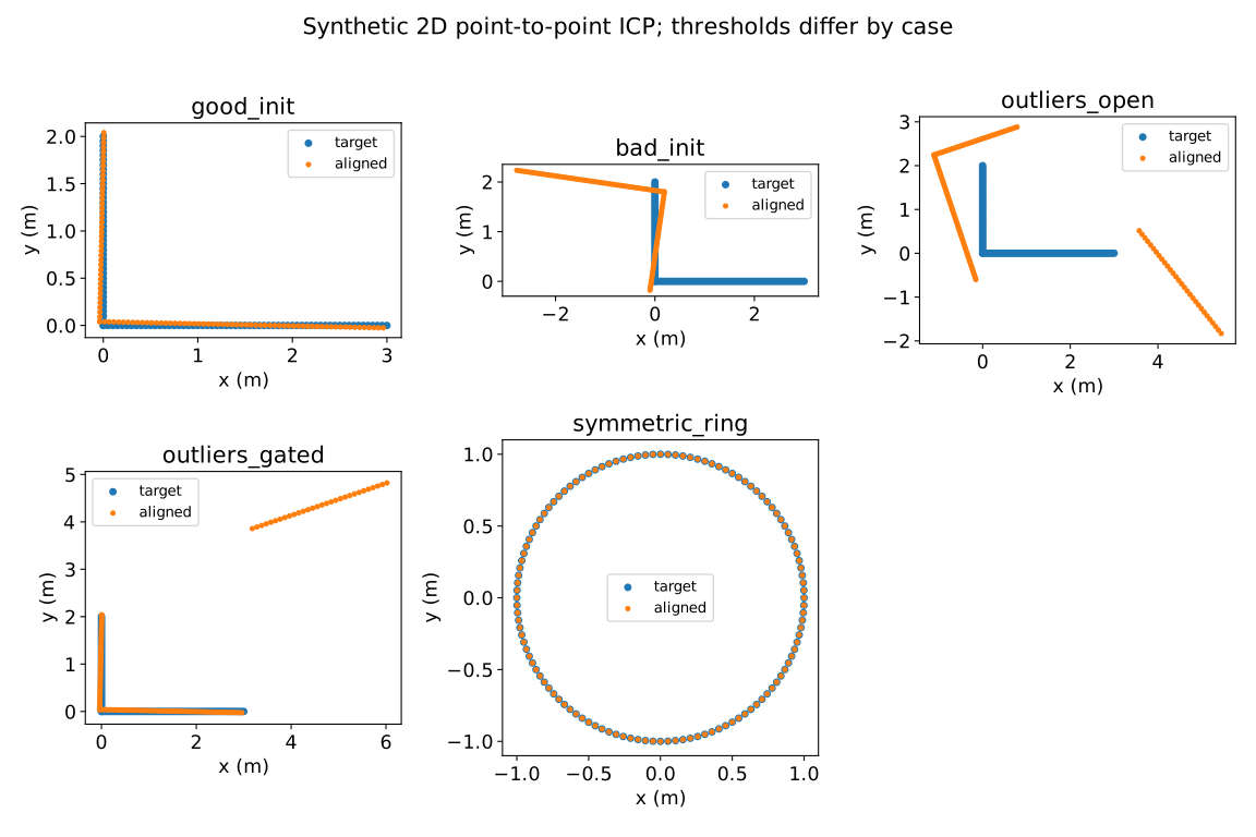
Even the good initialization leaves an error: neighboring points on regularly sampled segments permit a shifted local solution. Coverage 1.000 alone would miss it. Outliers lie at source x=4–7 m, y=3 m. Download the target, outlier input/output and summary.

Unobservable directions in circles and walls

The circle has radius 1 m and 120 points, with identity defined as the true transform. Its point set also matches after a 90° rotation, so essentially zero residual coexists with 90° pose error. More iterations cannot supply missing information.

A wall presents a related but different issue. Point-to-plane error measures displacement along the wall normal and poorly constrains tangential motion. Finite point-to-point walls can gain information from endpoints and point placement, but this becomes weak in a long corridor without visible endpoints. The circle is an executed experiment; the wall discussion explains the objective's directional constraints.

A smaller threshold is not a universal fix

The 0.5 m threshold removes these outliers, but can also eliminate correct correspondences when initialization is far away. Different thresholds select different points, so residuals alone are not directly comparable. This code stops updating with fewer than three accepted points; three points are not themselves a guarantee of good geometry.

Practical options include odometry initialization, coarse-to-fine alignment, outlier filtering and observing surfaces with different orientations. Measure their effects over the same intervals and reference conditions.

Continue to SLAM evaluation

This is single-frame 2D registration, not a test of 3D driving accuracy or moving-object robustness. SLAM evaluation adds trajectory errors, timing alignment and failed intervals. Vary only the initial angle first to see why convergence cannot be summarized by one residual value.

Run the same calculation locally

Extract the complete runnable source ZIP, or save the experiment entrypoint, generated kernels, and original PID source in one folder. PID uses the Python standard library; Kalman and ICP require NumPy. The original figure-generation commands remain available.

python3 -m pip install numpy==1.26.4
python3 experiment.py icp --parameters '{"case":"good_init","threshold":0.5}' > result.json

Try bad_init, outliers and symmetric_ring. Compare thresholds 10 and 0.5 for outliers. Verify that the ring can retain a 90-degree rotation error even with near-zero residual.