Contents — find the section you need
Background and reading guide
Background Basic frames, velocity and sensor terminology; use the reading guide for background.
Fundamentals · Explanations of principles, structure and trade-offs.
The spinning sensor on top of a self-driving car, or the small window on top of a robot vacuum — many of these are LiDAR (Light Detection And Ranging), a sensor that measures distance to its surroundings directly using laser light. LiDAR-SLAM is the technology that performs self-localization and mapping simultaneously using nothing but the point-cloud data a LiDAR returns (optionally aided by sensors such as an IMU). Where Visual-SLAM (see "Visual-SLAM Primer") tries to indirectly recover 3D structure from a camera's 2D images, LiDAR-SLAM starts with direct 3D distance information in hand — that's the key difference. This article starts from the principle of what a LiDAR actually measures, works through the two pillar algorithms for aligning point clouds — ICP and NDT — the feature-based design LOAM represents, Loop Closure and Graph SLAM, and finally the lineage of landmark algorithms and how to choose among them in practice. Current developments are covered in "Technology Trends in LiDAR-SLAM".
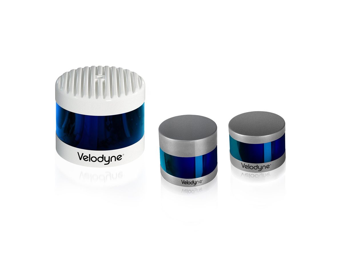 Velodyne LiDAR family
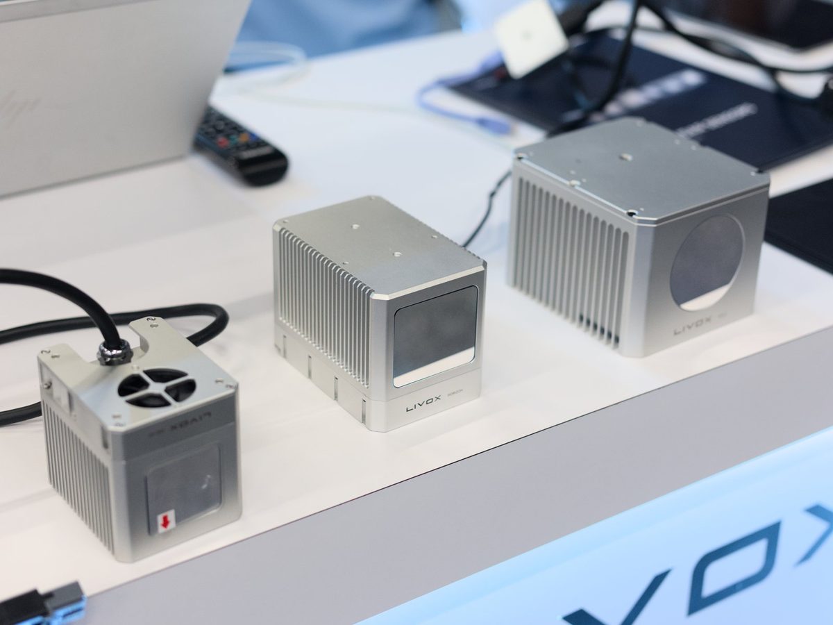 Livox LiDAR examples
Images: Velodyne Lidar sensor family (APJarvis, CC BY-SA 4.0) / Livox Mid-40, Horizon, and Tele-15 (Dllu, CC BY-SA 4.0), Wikimedia Commons. Representative product families, not necessarily the latest models named in the text.


0. What This Article Covers
- What a LiDAR actually measures, and why it obtains distance "directly"
- How the fundamental SLAM problem shows up in the world of point clouds
- How the two pillar scan-matching algorithms, ICP (Iterative Closest Point) and NDT (Normal Distributions Transform), work and how they differ
- The difference between the two modes of LiDAR Odometry, Scan-to-Scan and Scan-to-Map
- Why LOAM extracts features (edges and planes) at all, and the design thinking behind it
- How Loop Closure and Pose Graph optimization fit together
- The differences among landmark algorithms — ICP / NDT / LOAM / LeGO-LOAM / A-LOAM / Cartographer / LIO-SAM / FAST-LIO2 — and how to choose
1. What Is LiDAR-SLAM?
In one sentence: LiDAR-SLAM is the technology that uses the set of high-precision distance measurements (a point cloud) obtained from the time of flight (or phase shift) of laser light, repeatedly registering successive scans against each other (scan matching), to simultaneously estimate the sensor's own trajectory and a 3D map of its surroundings.
The input is the point cloud a LiDAR outputs at a fixed interval (anywhere from a few thousand to hundreds of thousands of points per scan), and the output — just as in Visual-SLAM — is two things: the sensor's 6-degree-of-freedom pose at each moment in time (3 for position, 3 for orientation), and a 3D point-cloud map of the surrounding environment. A self-driving car maintaining precise distance relationships to surrounding vehicles, pedestrians, and road infrastructure while estimating its own position; an autonomous mobile robot navigating precisely between warehouse shelves; a drone flying through geometrically complex spaces like tunnels or building interiors — LiDAR-SLAM is what's running under the hood in every one of these cases.
2. What Does a LiDAR Actually Measure?
LiDAR ranging principles fall into two broad categories. In the ToF (Time of Flight) approach, the sensor fires a laser pulse and measures the time T it takes for the reflection off the target to return, then derives distance D from the speed of light c.
Because the light travels the round trip, the measured time T has to be halved to get the one-way propagation time. The other approach, phase-shift (FMCW/AMCW), transmits a continuously modulated laser beam and derives distance from the phase difference between the transmitted and reflected signals. Either way, a LiDAR gets not just "there's something there" but the actual, absolute distance to it in a single observation — a capability a camera lacks entirely. As we'll see in section 4, a single monocular camera image can never recover real-world scale on its own, whereas a LiDAR point cloud carries metric scale from the outset.
There are also two families of LiDAR hardware. Mechanical spinning LiDAR rotates a stacked assembly of multiple laser transmitter/receiver elements to build a full 360-degree point cloud; Velodyne and Ouster are representative manufacturers. Solid-state LiDAR has no rotating mechanical parts, instead using MEMS mirrors or optical phased arrays to scan a limited field of view while achieving smaller size and lower cost; Livox is a representative example. Solid-state units trade a narrower field of view for, in many products, a non-repetitive scan pattern (scanning the same spot along a slightly different path every time), which means point clouds get denser the longer you accumulate them.
LiDAR point clouds also have a structure that camera images lack entirely. A spinning LiDAR fires multiple lasers stacked vertically (say, 16, 32, or 128 layers) while rotating horizontally, producing point clouds that are dense horizontally but sparse and layered vertically — an anisotropic distribution. This structure directly influences the design of LOAM's feature extraction and ICP's normal estimation, both of which we'll cover below.
3. The Fundamental SLAM Problem: "Where in the Map Does the Current Point Cloud Belong?"
Just as Visual-SLAM solves "where does the current image correspond, within past images and the map" by matching feature points, LiDAR-SLAM solves "where does the current scan (point cloud) correspond, within past scans and the map" by aligning point clouds against each other. The underlying problem is essentially the same regardless of sensor: a single observation alone can never determine absolute position; the only way forward is to keep estimating the current position using the correspondence with past observations (the map) as a clue.
What differs is the substance of that correspondence. Visual-SLAM detects "salient points" (features) in an image, numerically encodes the appearance around them as a descriptor, and searches for correspondences by descriptor similarity. A LiDAR point cloud, by contrast, carries almost no "appearance" information such as brightness or color to begin with (reflectance intensity is available, but it's far less discriminative than an image descriptor). As a result, matching point clouds is, in most cases, driven purely by spatial proximity — "which point is geometrically closest." The overall process of finding the rigid transform (rotation R, translation \mathbf{t}) between two point clouds is called Scan Matching, and it forms the core of LiDAR-SLAM.
The takeaway of this section is simple: where Visual-SLAM has "feature matching + Epipolar geometry," LiDAR-SLAM substitutes "scan matching." The next two sections cover the two pillar algorithms that realize scan matching: ICP and NDT.
4. Understanding ICP
ICP (Iterative Closest Point) is a classic algorithm for point-cloud registration, published by Besl & McKay in 1992 in IEEE Transactions on Pattern Analysis and Machine Intelligence, and still widely used today. As the name suggests, it's built on a simple idea: treat the "closest point" as the corresponding point, then refine that repeatedly.
The algorithm can be organized into three steps.
- Correspondence search: for each point p_i in the point cloud being moved (the source), find the closest point q_i in the fixed point cloud (the target) — typically using a spatial search structure such as a KD-tree.
- Transform estimation: given this set of correspondences \{(p_i, q_i)\}, find the rotation R and translation \mathbf{t} that minimize the sum of distances between corresponding points. The simplest version, the Point-to-Point error, is defined as follows.
- Apply and iterate: apply the resulting R and \mathbf{t} to the entire source point cloud, then go back to step 1 and search for correspondences again. This cycle of correspondence search → transform estimation → application repeats until the error becomes small enough (or stops decreasing).
Point-to-Point error is intuitive, but when aligning two broad, flat planes — a wall, say — it barely matters, from the error's perspective, exactly where along that plane the points correspond to each other (a small slide along the plane barely moves the error, as long as the perpendicular offset is small), so convergence tends to be slow. Point-to-Plane error solves this: it estimates a normal vector n_i from the local shape around the corresponding point q_i, and minimizes only the mismatch along the normal direction (the point-to-plane distance).
Point-to-Plane tolerates offsets along the plane while strictly penalizing only the mismatch perpendicular to it, and it's well known to converge faster and more stably than Point-to-Point, especially in plane-rich environments such as building interiors. That said, as noted in section 2, a spinning LiDAR's point cloud has a layered, vertically sparse structure, so naively estimating normals can produce noisy normals dragged around by the layering — normal estimation itself needs care.
ICP has two main weaknesses. First, since correspondence search relies purely on "nearest geometric neighbor," a large initial offset leads to incorrect correspondences and convergence to a local minimum — a good initial guess is required. Second, running nearest-neighbor search repeatedly over point clouds with tens of thousands of points per frame is computationally expensive, scaling with cloud size. NDT, covered next, takes a different approach that sidesteps correspondence search entirely.
5. Understanding NDT
NDT (Normal Distributions Transform) is a scan-matching algorithm with a fundamentally different approach from ICP, published by Biber & Straßer in 2003 at the IEEE/RSJ International Conference on Intelligent Robots and Systems (IROS). The original was proposed for 2D laser scanners; it was later extended to handle 3D point clouds as well.
The core idea of NDT is to represent a point cloud not as a set of individual points, but as a probability distribution defined per voxel on a regular grid. The distribution of points within each voxel is approximated as a Gaussian (normal distribution) with mean \mu and covariance matrix \Sigma.
Having represented the entire target point cloud this way — as a set of per-voxel Gaussian distributions forming a piecewise-continuous, differentiable probability density function — there's no longer any need to "search for point-to-point correspondences" in order to align the source cloud. Instead, for a transform T (rotation and translation) applied to each source point \mathbf{x}_i, giving \mathbf{x}_i' = T(\mathbf{x}_i), you sum up how "plausible" that transformed point is under the Gaussian of its corresponding voxel, as a score function, and find the T that maximizes it.
This optimization is solved with gradient-based methods such as Newton's method. Unlike ICP, there's no need to alternate between "correspondence search" and "transform estimation" as separate steps — you simply evaluate the gradient against the precomputed Gaussian parameters — so the cost of nearest-neighbor search is avoided entirely. And because the noise in individual points gets absorbed into a per-voxel mean and covariance, the result tends to be robust to noise.
NDT does come with its own trade-off, though: the choice of voxel size. Larger voxels are computationally lighter but average away fine shape differences, hurting alignment accuracy. Smaller voxels increase shape resolution but leave fewer points per voxel, making the Gaussian estimate itself unstable, and the growing voxel count raises computational cost as well. This tunable parameter that the user has to get right is what makes NDT practically fiddly to use.
6. LiDAR Odometry (Scan-to-Scan / Scan-to-Map)
The process of using ICP or NDT to find the relative motion between successive frames, and accumulating those estimates over time, is called LiDAR Odometry. As with Visual Odometry in Visual-SLAM, without some mechanism to reconcile with the map as a whole (Loop Closure), Drift accumulates over time and cannot be avoided.
LiDAR Odometry comes in two flavors depending on what it's compared against. Scan-to-Scan registers each scan only against the immediately preceding scan; it's computationally cheap, but because each estimation error carries straight into the initial guess for the next one, Drift tends to accumulate. Scan-to-Map registers the current scan not against a single previous scan but against the entire accumulated local map; drawing on more observations makes it less sensitive to noise and generally more accurate than Scan-to-Scan, at the cost of higher computation because the reference point cloud is larger.
Most practical LiDAR-SLAM implementations combine the two. A fast, coarse initial guess is obtained first — via Scan-to-Scan, IMU prediction, or a rough NDT-based alignment from section 5 — and that initial guess is then refined with a precise Scan-to-Map registration. The pipeline below illustrates a general LiDAR-SLAM processing flow built on this two-stage idea.
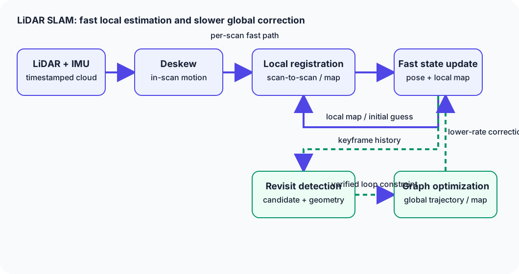
Figure 1 — The per-scan fast path runs from deskew through local registration to pose and local-map updates, feeding the next initial guess and reference map. A separate lower-rate path verifies revisits from keyframe history, admits loop constraints, and uses graph optimization to correct the global trajectory and map.
The Deskew step (correcting distortion during the scan) shown in the diagram is specific to LiDAR. A spinning LiDAR's single scan isn't captured instantaneously — it takes tens to a hundred-odd milliseconds to acquire. If the sensor itself moves during that window, points captured earlier and points captured later in the same scan end up representing observations from genuinely different times and positions, all mixed together within one scan (Motion Distortion). Deskew uses an IMU (or the previous velocity estimate) to correct for this motion during the scan, reconstructing the point cloud as though it had been captured from a single instant. This correction is deeply connected to the IMU fusion covered in VIO/LIO (see "VIO/LIO Primer").
7. Understanding LOAM
LOAM (Lidar Odometry and Mapping in Real-time), published by Zhang & Singh in 2014 at Robotics: Science and Systems (RSS), underlies the design of many LiDAR-SLAM implementations to this day. LOAM's central innovation is to extract only geometrically distinctive points instead of using every point in the cloud.
LOAM evaluates the local smoothness (curvature) around each point and extracts points with high curvature relative to their surroundings as edge features (sharp corners or outlines of objects), and points with low curvature as planar features (part of a smoothly continuing surface, such as a wall or floor). Instead of using an entire scan with tens of thousands of points for registration, narrowing it down to just these features drastically cuts the computational cost of scan matching.
Once the features are extracted, the error formulation echoes the ICP ideas from section 4, but the geometric element being matched against is a "line" or "plane" rather than a "point." An edge feature p_i is matched by minimizing its distance to the line spanned by two corresponding points p_a and p_b in the previous scan (or the map).
A planar feature is matched by minimizing its distance to the plane spanned by three corresponding points (the same form as the Point-to-Plane error in section 4). Summing these distances and minimizing over rotation and translation yields the relative motion between frames.
LOAM's other central design choice is its two-tier structure of high-frequency Lidar Odometry and low-frequency Lidar Mapping. Lidar Odometry runs a feature-based Scan-to-Scan match against the immediately preceding scan at high frequency (every scan), producing a coarse but fast pose estimate. Lidar Mapping takes that coarse estimate as its initial guess and runs Scan-to-Map matching against the accumulated map as a whole, at a lower frequency than Lidar Odometry, producing a more accurate pose and a more precise map. Running the two processes in parallel at different frequencies, with Lidar Mapping's result ultimately correcting Lidar Odometry's estimate, achieves both high-frequency output and high accuracy at once. This "high-frequency coarse estimate + low-frequency precise correction" design philosophy has been inherited by many of the later LiDAR-SLAM and LIO implementations covered in section 9.
8. Loop Closure and Graph SLAM
LiDAR Odometry alone accumulates Drift over time, just like Visual Odometry in Visual-SLAM, and even after a robot returns to its starting point, the estimated trajectory never notices. The mechanism that corrects this accumulated error is Loop Closure.
Loop Closure in the LiDAR world breaks down into two broad steps. First is Place Recognition: judging whether the current point cloud resembles a point cloud from a previously visited location. Since point clouds don't carry brightness information the way images do, this relies on approaches that encode the shape distribution of the point cloud itself as a descriptor — for instance, methods like Scan Context, which divide a scan into fan-shaped cells and encode the maximum height in each cell as a descriptor — or on methods that summarize geometric features of the whole point cloud. Second is geometric verification: for the scan pairs proposed as candidates by place recognition, actually attempting scan matching with ICP or NDT and checking whether they agree well enough. Only after passing both stages is a constraint linking "current position" and "position when that place was previously visited" trusted enough to be adopted.
Using this loop-closure constraint to correct the accumulated poses and map into a consistent whole is the job of Pose Graph optimization, or more generally, the Graph SLAM framework. It builds a graph whose nodes are the sensor's pose at each moment in time, and whose edges are constraints on relative motion between frames (or between two distant moments in time linked by a loop), then adjusts the nodes (poses) via nonlinear optimization so that all edge constraints are as mutually consistent as possible. The edge newly added by loop closure plays the role of redistributing Drift — which had until then only ever propagated in one direction — across the entire path that makes up the loop. This optimization, just as in Visual-SLAM (see "Visual-SLAM Primer", section 10), commonly relies on libraries such as g2o, GTSAM, and Ceres Solver inside LiDAR-SLAM implementations as well.
9. Landmark Algorithms
LiDAR-SLAM's history is easiest to follow along two axes: how point clouds get registered, and how far the design narrows things down to explicit features.
ICP (Besl & McKay, 1992) is, as covered in section 4, the classic and still widely used foundational algorithm for point-cloud registration. It's rarely used standalone for real-time SLAM, but some form of correspondence-based minimization derived from it lives on inside nearly every method that followed.
NDT (Biber & Straßer, 2003) is, as covered in section 5, Gaussian-distribution-based scan matching that avoids correspondence search, and stands alongside ICP as the other foundational choice, used broadly from 2D indoor robot SLAM to 3D autonomous-driving applications.
LOAM (Zhang & Singh, 2014) is, as covered in section 7, the method that introduced edge/plane feature extraction along with the two-tier high-frequency Odometry + low-frequency Mapping design, underlying the design of many LiDAR-SLAM and LIO implementations to this day.
LeGO-LOAM (Lightweight and Ground-Optimized Lidar Odometry and Mapping, Shan & Englot, published 2018 at the IEEE/RSJ International Conference on Intelligent Robots and Systems (IROS)) extends LOAM specifically for ground vehicles. It first separates the point cloud into ground and non-ground points, using ground points to estimate roll, pitch, and elevation, and non-ground points to estimate the remaining degrees of freedom (horizontal position and yaw), achieving a lightweight design capable of real-time operation even on embedded systems with limited compute.
A-LOAM (Advanced LOAM) is a simplified, open-source reimplementation of LOAM's ideas built on Ceres Solver-based nonlinear optimization, released by groups such as HKUST Aerial Robotics Group. It drops some of the fine-grained engineering tuning of the original LOAM in favor of clearer code, and is frequently referenced as an accessible implementation for learning and experimenting with the LOAM family of algorithms.
Cartographer (Hess, Kohler, Rapp, Andor, published 2016 at the IEEE International Conference on Robotics and Automation (ICRA), Google) performs Ceres Solver-based local scan matching on a per-submap basis (a submap being a bundle of several scans), combined with fast loop-closure detection via a divide-and-conquer Branch-and-Bound search over the candidate space. It supports both 2D and 3D, and — helped along by widely available open-source implementations for ROS — has been broadly adopted in indoor mapping.
LIO-SAM (Tightly-coupled Lidar Inertial Odometry via Smoothing and Mapping, Shan, Englot, Meyers, Wang, Ratti, Rus, published 2020 at IROS) is a tightly-coupled LiDAR-Inertial Odometry (LIO) method that jointly optimizes IMU preintegration factors, LiDAR-scan-matching odometry factors, GPS factors, and loop-closure factors within a shared Factor Graph (see "VIO/LIO Primer" for details).
FAST-LIO2, published by Xu, Zhang, and colleagues at the University of Hong Kong's MARS Lab, is a fast LIO built on a Tightly-Coupled Iterated Kalman Filter. By managing the point cloud directly with a sequential nearest-neighbor search structure (an incremental k-d tree, iKD-Tree), it registers the point cloud directly against the map without an explicit feature-extraction step, and its design prioritizes real-time operation on small platforms with limited compute. Current 2026-vintage developments are covered in "Technology Trends in LiDAR-SLAM".
10. Comparing the Methods
| Method | Principle | Accuracy | Compute cost | Robustness | Implementation difficulty |
|---|---|---|---|---|---|
| ICP | Nearest-neighbor search + iterative rigid-transform minimization | High accuracy given a good initial guess; falls into local minima otherwise | Medium–high (iterative nearest-neighbor search cost) | Weak in geometrically featureless environments or against large initial offsets | Low (conceptually simple, many existing implementations) |
| NDT | Maximizing fit against per-voxel Gaussian distributions | Depends on voxel size; comparatively robust to noise | Medium (no correspondence search, but gradient computation involved) | Robust to noise but requires voxel-size tuning | Medium (tuning takes some knack) |
| LOAM | Edge/planar feature extraction + two-tier Odometry/Mapping | High accuracy in feature-rich environments | Medium (lighter than using the whole point cloud, thanks to feature selection) | Weak in feature-poor environments (tunnels, etc.) | Medium–high (complex parameters and design) |
| LeGO-LOAM | Ground-point separation + LOAM-style two-tier optimization | High accuracy for ground vehicles; assumptions break down for aerial platforms | Medium (lighter than LOAM) | Strongly dependent on the presence of a flat ground plane | Medium |
| A-LOAM | Simplified reimplementation of LOAM using Ceres Solver | Roughly LOAM-equivalent (varies by implementation) | Medium | Inherits LOAM's same weaknesses | Low–medium (easy to reference for learning) |
| Cartographer | Per-submap scan matching + Branch-and-Bound loop closure | High accuracy indoors (2D); strong on global consistency | Medium–high (submap management and Branch-and-Bound search cost) | Strong in loop-rich indoor environments | Medium (easy to adopt within the ROS ecosystem) |
| LIO-SAM | Factor-graph optimization of IMU preintegration + LiDAR odometry + GPS + loop closure | High accuracy with IMU fusion; global consistency improves further with GPS | High (factor-graph optimization cost) | IMU helps counter geometric degeneracy | Medium–high (specific sensor assumptions, e.g. 9-axis IMU) |
| FAST-LIO2 | Direct registration via Iterated Kalman Filter + iKD-Tree | High accuracy at high frequency (especially pronounced on solid-state LiDAR) | Low–medium (direct method avoids feature-extraction cost) | Depends on IMU under degeneracy; weak under extreme low-geometry conditions | Medium (implementation is public, but internal tuning requires expertise) |
Overall, it helps to see ICP and NDT as the "foundational registration algorithms," the LOAM family (LOAM/LeGO-LOAM/A-LOAM) as "efficiency gains through feature design," Cartographer as "efficient global consistency and loop closure," and LIO-SAM/FAST-LIO2 as "robustness gains through tight IMU coupling" — each a distinct axis of improvement built on what came before.
11. Where LiDAR-SLAM Struggles
Because LiDAR actively emits laser light to measure distance, it holds up well against darkness and backlighting — the environments where Visual-SLAM struggles. But LiDAR-SLAM has weaknesses of its own.
- Geometric degeneracy: in environments where the point-cloud shape barely changes along a particular direction — a long tunnel, or a broad, flat parking lot — scan matching can't uniquely determine translation or rotation along that direction. This happens because the ICP/NDT optimization lands in a "flat valley" where the error barely changes for any value along that direction; it shares the same underlying root cause as the weakness Visual-SLAM has against featureless walls.
- Severe weather: rain, snow, fog, and dust scatter and absorb laser light, attenuating reflections that would otherwise return, or generating noise points (spurious reflections that appear at positions where nothing actually exists).
- Mirrors and transparent objects: glass and mirrors can specularly reflect laser light, generating spurious points at a location other than the actual object's position (the mirror-image location).
- Dynamic objects: using points on moving objects — pedestrians, vehicles — as though they were part of a static environment during registration introduces error into the estimate of the sensor's own motion. Detecting and excluding dynamic objects, or explicitly modeling them, becomes necessary.
- The point-density-vs-compute-cost trade-off: higher-resolution, higher-frequency point clouds tend to yield more accurate registration, but the more points per frame, the higher the computational cost of scan matching. In embedded systems or drones with limited compute, this trade-off between density and speed becomes a major design constraint.
- Hardware cost: high-resolution, long-range spinning LiDARs remain substantially more expensive than cameras, and cost is often a real barrier to adoption.
Many of these weaknesses cut in a different direction from a camera's weaknesses, which makes combining Camera (Visual-SLAM) and LiDAR (LiDAR-SLAM) — sensor fusion (see "Sensor Fusion Primer") — a powerful way to compensate for the limits of either sensor alone.
12. Choosing in Practice
How to choose among LiDAR-SLAM methods depends heavily on what sensors can be mounted, available compute, required accuracy, and the geometric character of the environment.
- Indoor service robots and robot vacuums: low-cost 2D LiDAR remains a strong, persistent choice, and robust 2D SLAM implementations like Cartographer are widely used. Indoor spaces, rich in structures such as walls and furniture, rarely encounter geometric degeneracy, making them a favorable environment for LiDAR-SLAM.
- Self-driving cars: high-resolution 3D LiDAR combined with multi-sensor fusion across GPS, IMU, and camera is the baseline assumption. To counter geometrically degenerate stretches like tunnels and overpasses, tightly IMU-coupled configurations like LIO-SAM/FAST-LIO2 carry significant weight.
- Drones: given tight weight and power constraints, solid-state LiDAR (e.g., Livox) paired with a compute-efficient direct method like FAST-LIO2 tends to be favored.
- Warehouse and factory AGVs/AMRs: environments with regular, corridor-like structure are common, making 2D LiDAR-based Scan-to-Map approaches (e.g., Cartographer) a practical choice. In environments where shelf layouts change frequently, map update frequency also factors into the selection.
- Degenerate environments — tunnels, underground spaces, long straight corridors: LiDAR alone tends toward unstable registration, so tight IMU coupling (LIO-SAM/FAST-LIO2) or combining with an independent source like wheel odometry becomes practically essential.
- Indoor vs. outdoor: indoor spaces are structure-rich with abundant geometric cues, favoring LiDAR-SLAM, while outdoor spaces raise the challenge of degeneracy in open areas and severe weather, making IMU/GNSS fusion more important.
As a practical rule of thumb: a direct method like FAST-LIO2 for constrained compute and high-frequency output, LIO-SAM for global consistency that also incorporates GPS, and Cartographer for a track record in 2D environments and tight integration with the ROS ecosystem. A configuration with no IMU at all (ICP/NDT/LOAM standalone) has become an almost impractical choice today given the demand for resilience to degenerate environments, and most operational systems are now designed around tight IMU coupling as a baseline assumption.
13. References
- Besl & McKay, “A Method for Registration of 3-D Shapes” (IEEE TPAMI, 1992)
- Zhang & Singh, “LOAM: Lidar Odometry and Mapping in Real-time” (RSS, 2014)
- Xu et al., “FAST-LIO2: Fast Direct LiDAR-Inertial Odometry” (IEEE T-RO, 2022)
14. Summary
LiDAR-SLAM takes the metric-scale distance information (point clouds) obtained from a laser's time of flight, performs scan matching with either ICP (iterative registration of nearest points) or NDT (fitting to per-voxel Gaussian distributions), accumulates a trajectory through LiDAR Odometry combining Scan-to-Scan and Scan-to-Map, and keeps correcting accumulated error through Loop Closure and Pose Graph optimization — together achieving simultaneous self-localization and mapping. The lineage of landmark algorithms — the LOAM family (efficiency through feature extraction), Cartographer (efficient global consistency), and LIO-SAM/FAST-LIO2 (robustness through tight IMU coupling) — each evolved as an answer to a distinct challenge, and on the single point of coping with geometrically degenerate environments, most operational systems have converged on designs built around tight IMU coupling as a baseline.
Does successful ranging uniquely determine LiDAR pose?
Planes and long corridors can leave some motion directions weakly constrained. Ranging success and registration observability are different.
Comments
Please log in to post a comment
No comments yet.