Contents — find the section you need
Background and reading guide
Background Basic vectors, matrices and camera projection.
Fundamentals · Explanations of principles, structure and trade-offs.
Robot vacuums, drones, self-driving cars, and AR glasses all share one requirement: answering the question "where am I right now?" GPS doesn't work indoors or in dense cities, and a map isn't always available to begin with. Visual-SLAM is the technology that answers this question using camera images alone (sometimes paired with cheap auxiliary sensors). This article starts from why a robot loses track of its own position in the first place, then works through feature tracking, the math of camera geometry, the difference between Visual Odometry and SLAM, the lineage of landmark algorithms, and finally how to choose one in practice.
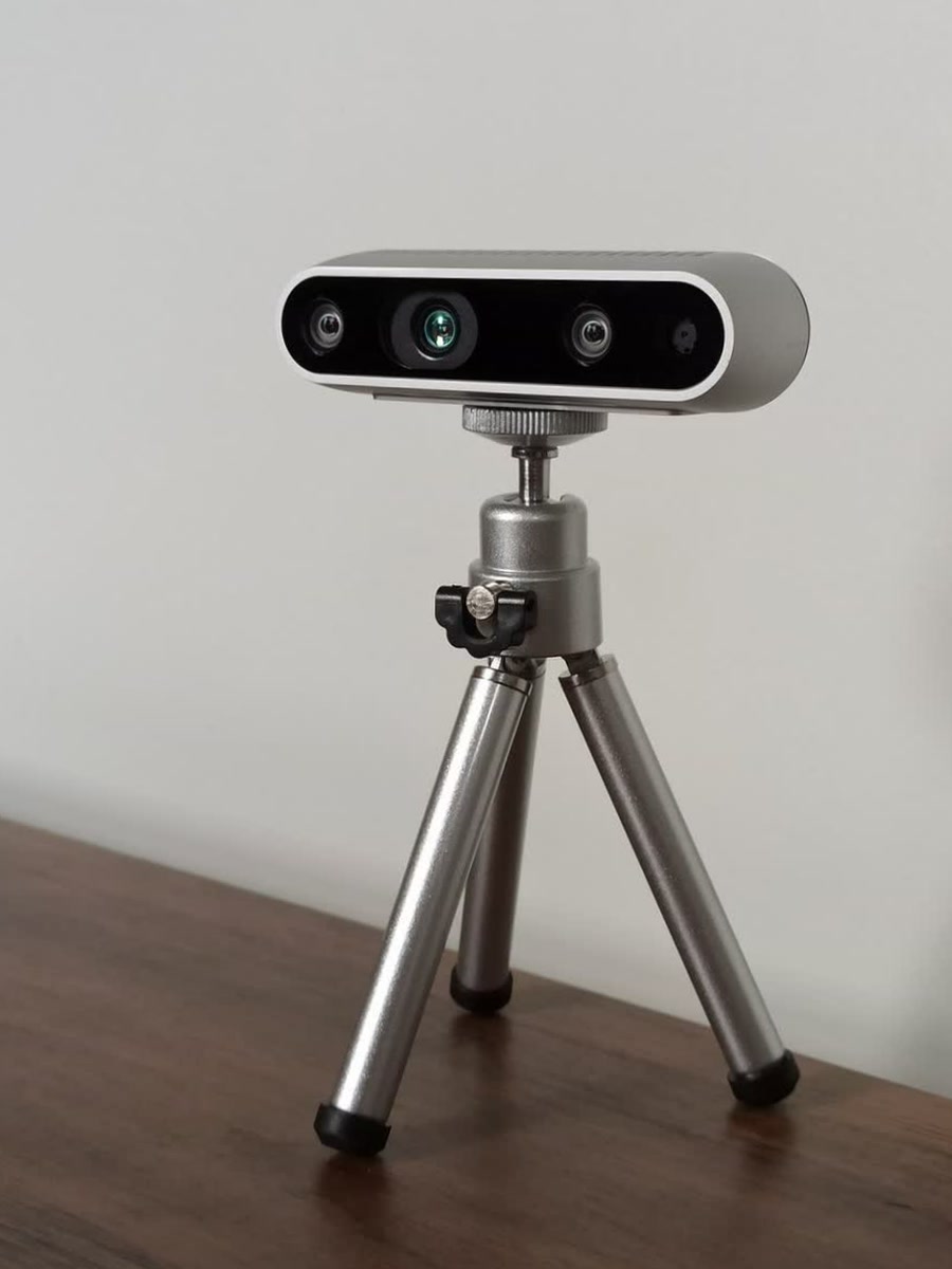 Visual-SLAM input camera
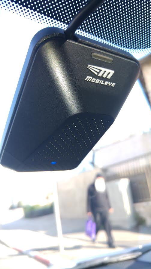 Vehicle camera example
Images: Intel RealSense depth camera D435 (Marc Auledas, CC BY-SA 4.0) / Car window camera of Mobileye system (Ranbar, CC BY-SA 4.0), Wikimedia Commons. Representative cameras, not a required Visual-SLAM hardware configuration.


0. What This Article Covers
- What Visual-SLAM is, and why a camera alone can estimate its own position
- How Visual Odometry (VO) differs from SLAM
- What ORB-SLAM, LSD-SLAM, DSO, SVO, and DROID-SLAM each contribute as design choices
- The difference between Feature-based, Direct, and Learning-based approaches
- Where Visual-SLAM struggles, and why
- How to actually choose a method for a robot, a drone, AR/VR, or a self-driving car
1. What Visual-SLAM Actually Does
In one sentence: Visual-SLAM estimates a camera's own trajectory through space (Localization) and the 3D structure of its surroundings (Mapping) simultaneously, using nothing but the sequence of images the camera captures.
The name itself — Simultaneous Localization And Mapping — points to what matters most: the word "simultaneous." If the map were already known, finding your own position would be a comparatively easy problem; if your position were already known precisely, building the map would be easy too. Visual-SLAM faces neither luxury — building the map requires knowing your position, and knowing your position requires the map. This chicken-and-egg dependency has to be untangled from the same stream of observations, at the same time.
The input is a time series of images from a camera (monocular, stereo, or RGB-D), and the output is two things: the camera's 6-degree-of-freedom pose (3 for position, 3 for orientation) at every timestep, and a map representing the surroundings (a sparse set of feature points, or a dense 3D shape). A robot vacuum learning a room's layout while it cleans, a drone stabilizing its hover indoors or underground where GPS never reaches, an AR headset overlaying virtual objects onto the real world without drift — in every one of these cases, Visual-SLAM is running underneath.
2. Why Doesn't a Robot Know Where It Is?
To understand the problem Visual-SLAM actually solves, it helps to ask concretely: why does a robot lose track of its own position in the first place?
First, there are plenty of environments with no GPS, or no GPS worth trusting. Indoors, underground, in tunnels, in the urban canyons between skyscrapers (where multipath reflections blow up positioning error), or underwater and on other planets where a satellite constellation doesn't even exist — none of these give you a way to obtain an absolute position directly.
Second, there's the problem of a map simply not existing. A newly built structure, a disaster site, an unexplored planetary surface — pre-built map data isn't always available. Without a map, "check your position against the map" isn't even an option.
Third — and most fundamentally — a single sensor reading can't determine absolute position, even in principle. A camera only tells you what's around it right now. Looking at one image doesn't instantly tell you "this is 2.3 meters from that wall, in the living room" — recognizing that wall as "that wall" requires having seen it before, and remembering where you were when you did. In other words, turning a current observation into meaningful position information requires a correspondence with past observations (where you are now depends on where you've been) — and that correspondence is exactly what a map provides.
The essence of the SLAM problem is building this correspondence between "what I see now" and "what I've mapped before," continuously and consistently, from observation data alone, with no external absolute position ever provided. A single mistaken correspondence propagates its error into every estimate that follows — and how to suppress this accumulated error, and how to correct it after the fact, is the central design question behind every Visual-SLAM algorithm.
3. What to Find in a Camera Image
A camera's raw output is nothing more than a grid of pixel values — brightness, color. The first step toward figuring out "how did I move" is finding trackable cues inside that grid.
A Feature is a local point in the image that stands out clearly from its surroundings and can be reliably re-detected even as the viewpoint changes — a corner, an edge intersection, a place where brightness gradients change sharply in multiple directions. A uniform patch of blue sky, indistinguishable from its neighbors, can't serve as a feature.
Feature Detection finds candidate feature points within a single image. Algorithms like ORB (Oriented FAST and Rotated BRIEF), SIFT, and the FAST corner detector decide which pixels "look like" features, and compute a descriptor — a numerical summary of the local appearance around each one.
Feature Tracking finds and matches those same features across the next frame in time. There are two broad approaches: matching detected features by descriptor similarity (Feature Matching), and starting from a feature's position in the previous frame and searching its neighborhood in the next frame (Optical Flow, classically via the Lucas-Kanade method).
This relationship — the same point in the real world appearing at different locations across different frames — is called a Correspondence. Nearly every geometric computation in Visual-SLAM takes a set of correspondences as its input; without a single correspondence, there is, in principle, no clue at all about how the camera moved.
Optical Flow is a vector field describing how far, and in what direction, each point in the image (or a sparse set of points) moved between frames — not just features. Where feature-based tracking follows only the most distinctive points, optical flow can exploit motion information over a wider area, at generally higher computational cost.
4. Computing the Camera's Motion
Once correspondences are in hand, they can be turned, geometrically, into an estimate of how the camera moved. The foundation for that computation is Epipolar Geometry.
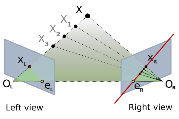
Figure 1 — Two camera viewpoints O_1 and O_2, a point X in space, and its projections x_1, x_2 onto each image plane. Given x_1, its corresponding point x_2 is always constrained to lie on a single line in the second image (the epipolar line).
Figure: Epipolar geometry (Arne Nordmann, CC BY-SA 3.0 / GFDL), Wikimedia Commons. The original SVG is converted to a white-background PNG for reliable browser display.

When the same point X in space is photographed from two different viewpoints, the corresponding point \mathbf{x}_2 in one image, given a point \mathbf{x}_1 in the other, isn't free to be anywhere in the image — it must lie on a single line (the epipolar line). The matrix encoding this geometric constraint is the Essential Matrix E. When the camera's intrinsic parameters are known, corresponding points in normalized camera coordinates satisfy:
Here R and \mathbf{t} are the rotation and translation from camera 1 to camera 2, and [\mathbf{t}]_{\times} is the skew-symmetric matrix built from \mathbf{t} that represents a cross product as a matrix multiplication. This equation says that this constraint always holds among a correspondence \mathbf{x}_1, \mathbf{x}_2, and the camera's relative rotation and translation. The required number of correspondences depends on the estimator: a calibrated Essential Matrix has a 5-point minimal solver, while linear 8-point estimation uses at least 8 correspondences. Real data contain outliers, so practical systems collect more matches and combine them with RANSAC or another robust estimator. When intrinsics are unknown, or when working directly in pixel coordinates, the Fundamental Matrix F = K_2^{-\top} E K_1^{-1}, which folds in the intrinsic matrix K, plays the same role.
The translation \mathbf{t} recovered from the Essential Matrix carries no real-world unit (meters, say) — two images alone can't tell you whether the camera moved one meter or two. This scale ambiguity is a constraint specific to Visual-SLAM, particularly monocular configurations, and is revisited in Section 5.
Computing the actual 3D position of a correspondence — the coordinates of the point X in space — is called Triangulation. Extending the two rays that go from each viewpoint toward X, those two rays should, ideally, intersect at exactly the point X; finding that intersection recovers the 3D position of the correspondence (in practice, observation noise means the rays don't exactly meet, so the point closest to both, in a least-squares sense, is found instead).
If a correspondence is available between a landmark whose 3D position is already known and where it appears in the image, the camera's pose can be computed directly from that. This is the PnP (Perspective-n-Point) problem: given n 3D points and their projected positions in the image, solve for the camera's position and orientation. Once a map already exists, PnP becomes the central tool for computing each new frame's camera pose.
5. Visual Odometry
Simply repeating "compute the camera's motion from correspondences," frame after frame, is already enough to estimate the camera's trajectory. This is Visual Odometry (VO).
VO stitches together only the relative motion between the current frame and the previous one (or the last few frames) to build up the camera's trajectory. It generally has no mechanism for maintaining a persistent map or for recognizing a previously visited place — it's closer in spirit to a car's odometer, continuously computing "how far have I moved since just now."
The distinction between VO and SLAM lies precisely in this: whether the system maintains a map and has a mechanism for recovering consistency with the past. VO is lightweight and simple to implement, but because each frame's estimate always depends on the previous one, small errors accumulate without bound over time. This accumulated error is called Drift. If a robot loops back to its starting point, VO alone has no way of recognizing "I'm back where I started" — the estimated trajectory stays offset from the start and never closes.
There's another problem specific to VO, especially monocular VO, that Section 4 already touched on: the Scale problem. Images from a monocular camera alone can't recover an absolute real-world unit of length — nothing in the image's appearance distinguishes "moved 2 meters, object appears twice as large" from "moved 4 meters, object appears four times as large." A stereo camera (which has a known baseline distance between its two lenses to anchor scale), an RGB-D camera (whose depth sensor gives real-world distances directly), or pairing with an IMU (whose real-scale acceleration lets scale be estimated) can resolve this scale ambiguity.
6. What SLAM Adds on Top of VO
It helps to think of SLAM as VO plus the following additional pieces.
A Map is an accumulated representation of every feature's 3D position observed so far (or a dense 3D shape). Rather than comparing only against the immediately preceding frame, as VO does, the system can now match against everything accumulated in the map.
A Landmark is an individual element of that map — usually a feature point with a 3D position. Every time a new frame arrives, matching it against the landmarks visible in that frame lets the system estimate the camera pose consistently not just with the previous frame, but with the entire map built up over the robot's history.
Loop Closure is SLAM's single most important advantage over VO. When a robot returns to a place it has visited before, image similarity is used to detect that fact, and a new constraint is added to the map linking "where I am now" to "where I was when I first visited this place." Adding this constraint lets the system redistribute the drift accumulated along the entire loop and correct it.
The result of that correction is Global Consistency. Before loop closure, accumulated error means two positions in the map that should really be the same physical place end up recorded as slightly different locations. Loop closure correction detects that discrepancy and reshapes the whole map into a self-consistent form — this loop closure mechanism is exactly why SLAM can offer not just "a record of motion" but "a consistent map."
7. The Basic Structure of Visual-SLAM
Putting these pieces together reveals a pipeline shared, in broad strokes, by every major modern Visual-SLAM system.
Figure 2 — Images from the Camera are matched against the previous frame (Feature/Direct Tracking, using one of the approaches from Sections 3 and 8), which drives Pose Estimation (epipolar geometry and PnP from Section 4) and, in parallel, Local Mapping (adding and updating landmarks in the recently observed area). When a loop is detected, Loop Closing fires, and the Optimization layer in the Backend (Section 10) — Bundle Adjustment or Pose Graph optimization — corrects the accumulated poses and map into a consistent whole.
Images from the Camera first go through Feature/Direct Tracking (either of the approaches covered in Sections 3 and 8) to establish correspondences with the previous frame. From these correspondences, Pose Estimation (using the epipolar geometry and PnP from Section 4) computes the camera pose, while Local Mapping (adding and updating landmarks in the recently observed region) proceeds in parallel. When a loop is detected, Loop Closing fires, and the Backend's (Section 10) Optimization stage corrects the accumulated poses and map into a globally consistent whole. The end result of this pipeline is the final output: the camera's Pose (trajectory) and Map (the 3D structure of its surroundings).
8. Landmark Algorithms
The history of Visual-SLAM is easiest to follow along one axis: how much is designed explicitly, and how much is handed off to learning.
PTAM (Parallel Tracking and Mapping, Klein & Murray, 2007) was a pioneering system that ran Tracking (pose estimation) and Mapping (map building) as separate parallel threads. Tracking runs fast, every frame, while the computationally expensive Bundle Adjustment for Mapping runs in a background thread with more time to spare — this idea of splitting Tracking from Mapping was inherited by many later Visual-SLAM systems.
ORB-SLAM (Mur-Artal, Montiel & Tardós, 2015) built around ORB features, combining a three-thread structure (Tracking, Local Mapping, Loop Closing) with Place Recognition (matching against past frames via Bag-of-Words) to achieve practical monocular performance. ORB-SLAM2 (Mur-Artal & Tardós, 2017) extended that framework beyond monocular to stereo and RGB-D cameras. ORB-SLAM3 (Campos, Elvira, Gómez Rodríguez, Montiel & Tardós, 2021) added tight coupling with an IMU (Visual-Inertial SLAM) and Multi-Map SLAM, which maintains multiple maps and merges them as needed — and remains, to this day, the de facto reference implementation for feature-based SLAM.
LSD-SLAM (Large-Scale Direct monocular SLAM, Engel, Schöps & Cremers, 2014) is a landmark example of the Direct method, showing that camera pose can be estimated using image brightness directly, with no feature detection step, at large scale. Skipping feature extraction altogether lets it exploit information even where features are sparse.
DSO (Direct Sparse Odometry, Engel, Koltun & Cremers, first presented in 2016, published 2018) stays direct, but rather than the semi-dense estimate LSD-SLAM produces, it minimizes photometric error over a sparse set of points, achieving both accuracy and computational efficiency.
SVO (Fast Semi-Direct Monocular Visual Odometry, Forster, Pizzoli & Scaramuzza, 2014) combines feature detection with a direct method in a semi-direct approach, tracking brightness in patches around detected features to achieve fast operation at high frame rates — designed with resource-constrained platforms like drones in mind.
DROID-SLAM (Teed & Deng, 2021) replaces the explicit feature extraction and matching step entirely with deep learning, estimating camera pose and per-pixel depth via a correlation volume, a recurrent update operator, and a differentiable Bundle Adjustment layer — the representative Learning-based approach (its internal mechanics are covered in more detail in Visual-SLAM Trends).
9. Feature-based vs. Direct vs. Learning-based
Boiled down, these algorithms fall into one of three design philosophies.
| Aspect | Feature-based (e.g. ORB-SLAM3) | Direct (e.g. DSO/LSD-SLAM) | Learning-based (e.g. DROID-SLAM) |
|---|---|---|---|
| Principle | Detects and describes features, computes pose from the geometric relationship among correspondences | Skips features entirely, minimizes image brightness directly to find pose | A neural network learns to replace feature extraction, correspondence, and pose/depth estimation |
| Accuracy | High where features are plentiful; tends to produce a sparse map | Works wherever there's a brightness gradient; can produce semi-dense to dense maps | Reasonably robust even in low-texture environments; easy to get dense depth |
| Compute cost | Moderate (feature extraction, descriptors, matching) | Varies by implementation, generally lightweight (DSO in particular optimizes for efficiency) | High (inference alone often needs several to over a dozen GB of GPU memory) |
| Robustness | Weak in low-texture environments or with dynamic objects; comparatively strong against lighting change | Sensitive to brightness changes (auto-exposure, lighting) | Strong within the range of its training data, but generalization to unseen environments can be limited |
| Implementation difficulty | Many mature open-source implementations, easy to adopt | Mathematics (linearizing brightness) is somewhat more involved | Easy to use a pretrained model; retraining or tuning internals requires more expertise |
Feature-based methods have the longest track record, including plenty of embedded deployments; Direct methods hold up better where texture is scarce; Learning-based methods are improving fast but demand heavier compute — that's roughly the current landscape as of 2026.
10. The Backend
What ultimately determines Visual-SLAM's accuracy isn't just the frontend (feature extraction, tracking, pose estimation) — it's the Backend, which polishes the entire accumulated set of observations into something self-consistent.
Bundle Adjustment jointly optimizes camera poses and the 3D positions of landmarks so that they're maximally consistent with every observation. It minimizes the total reprojection error — the discrepancy between a landmark \mathbf{X}_i projected into an image via camera pose (R_j, \mathbf{t}_j) and where the corresponding feature was actually observed, \mathbf{u}_{ij}.
\pi(\cdot) is the projection function from a 3D point to the image plane, based on the camera's intrinsic parameters. Global Bundle Adjustment, which optimizes every frame and every landmark simultaneously, is highly accurate but expensive; in practice it's typically paired with Local Bundle Adjustment, restricted to just the most recent handful of frames, to keep computation manageable.
When a loop closure is detected, Pose Graph optimization comes into play. Unlike Bundle Adjustment, which includes every landmark, Pose Graph optimization treats only the camera's pose at each timestep as a node, with edges encoding relative-pose constraints between frames — optimizing pose alone, quickly. The new constraint added by loop closure redistributes the accumulated drift across the whole loop.
Both of these are solved within the framework of Nonlinear Optimization. Because the projection function \pi(\cdot) and the composition of rotations in a pose are inherently nonlinear, iterative methods like Gauss-Newton and Levenberg-Marquardt are used, and libraries like g2o and Ceres Solver are widely relied on inside Visual-SLAM implementations.
11. Where Visual-SLAM Struggles
Because Visual-SLAM depends on a passive sensor — a camera — its accuracy degrades systematically in a handful of situations.
- Darkness: Without enough light, the image's signal-to-noise ratio degrades, destabilizing both feature detection and the brightness-gradient computations that direct methods rely on. Infrared-illuminated RGB-D cameras can compensate somewhat, but the effect is limited outdoors at night.
- Low texture: White walls, plain floors, glass surfaces — anywhere brightness gradients are scarce, features can't be found, or the direct method's minimization becomes ill-posed and prone to local minima.
- Fast motion: Rapid camera movement or rotation widens the search range needed to find correspondences between frames, and combined with motion blur (below), tracking easily breaks down. Pairing with an IMU (VIO) is the standard way to compensate for this weakness.
- Dynamic objects: Treating features on a moving pedestrian or car as if they belonged to the static environment injects error into the estimate of the camera's own motion. This requires either preprocessing to detect and exclude dynamic objects, or extensions that model them explicitly.
- Motion Blur: Blurring caused by camera or subject motion during the exposure window, which destabilizes feature descriptors and degrades matching accuracy. Global-shutter cameras or high-light environments with short exposure times reduce the impact.
All of these share a common thread: the camera simply isn't getting enough visual information to work with. An active ranging sensor like LiDAR (see LiDAR-SLAM Technology Trends) sidesteps most of these weaknesses in principle, but carries its own set of weaknesses (see Section 2) — no single sensor is universally sufficient, and that complementarity is exactly why Sensor Fusion (see the Sensor Fusion Primer) matters.
12. Choosing a Method in Practice
How to pick a Visual-SLAM approach depends heavily on what sensors you can carry, how much compute is available, and what accuracy and real-time performance the application demands.
- Robots (indoor service robots, cleaning robots): Often constrained to low-cost camera setups, where feature-based ORB-SLAM-family methods or dense mapping via RGB-D cameras are practical choices. In corridor-heavy, low-texture environments, pairing with LiDAR is worth considering.
- Drones: Severe constraints on compute and payload weight push toward lightweight semi-direct methods like SVO, or tightly-coupled VIO configurations with an IMU.
- AR/VR: Real-time performance and low latency are the top priority, and a Visual-Inertial configuration paired with the headset's built-in IMU has become the de facto standard. In AR specifically, Global Consistency directly determines whether virtual objects drift, so loop closure accuracy matters a great deal too.
- Autonomous driving: Rarely used as standalone Visual-SLAM; camera-based visual information is typically folded into a multi-sensor fusion setup alongside LiDAR, radar, and GNSS (see the Sensor Fusion Primer).
- Indoor vs. outdoor: Indoors, lighting changes are gentle and there's plenty of structure, so feature-based methods tend to work well; outdoors, lighting variation, dynamic objects, and vast scale become challenges, making the robustness of loop closure that much more important.
As of 2026, the rough decision axis looks like this: choose Learning-based if compute is abundant and top accuracy is the goal, Feature-based if embedded track record and low resource use matter most, and Direct if resilience in texture-poor environments is essential. The latest research directions — reshaping map representation with 3D Gaussian Splatting/NeRF, feed-forward 3D foundation models, and more — are covered in Visual-SLAM Trends.
Five checks before implementation
Choosing by algorithm name alone makes failures in the field difficult to diagnose. Before implementation, make sure these five items can be logged; when tracking fails, you can then separate a sensor problem from an estimator problem.
| Check | Information to prepare | What goes wrong if it is missed |
|---|---|---|
| Calibration | Intrinsics K, lens distortion, and the stereo baseline if applicable | Reprojection error looks like pose error, and scale cannot be evaluated |
| Time synchronization | Frame timestamps, camera–IMU offset, and dropped frames | During fast motion, the image and inertial data describe different poses |
| Shutter and exposure | Global/rolling shutter, exposure time, and auto-exposure settings | Motion blur or geometric distortion is mistaken for an algorithm failure |
| Dynamic objects | Whether masks are used, the fraction of moving objects, and rejected correspondences | Pedestrians or vehicles are absorbed into the static map |
| Evaluation logs | Ground truth, ATE/RPE, track-loss times, and loop-detection results | “It moved” is not enough to compare accuracy, drift, or recovery |
Filling in this table first also makes it easier to separate what must change and what can stay fixed when switching from Feature-based to Direct or Learning-based methods. Visual-SLAM should be selected as a system — camera, timing, preprocessing, optimization, and evaluation included — rather than as an algorithm in isolation.
13. Summary
Visual-SLAM tracks correspondences from camera images alone, recovers the camera's motion via epipolar geometry and PnP, and continuously corrects accumulated error through a map and loop closure — achieving simultaneous localization and mapping. The three design philosophies — Feature-based (the ORB-SLAM family), Direct (DSO/LSD-SLAM), and Learning-based (DROID-SLAM) — each rest on a different tradeoff, and are easiest to understand along the axes of whether features are handled explicitly, whether brightness is used directly, and how much is delegated to learning. Which one to actually pick is an application-specific judgment call, balanced against available sensors, compute, and the required accuracy and real-time performance.
14. References
The primary papers and research pages for the representative methods and two-view geometry discussed above are collected here as starting points for implementation and further reading. To avoid confusing a paper's claim with performance on a particular product or dataset, read the linked text together with its experimental conditions.
- ORB-SLAM3: An Accurate Open-Source Library for Visual, Visual-Inertial and Multi-Map SLAM — one library covering visual, visual-inertial, and multi-map designs.
- DROID-SLAM: Deep Visual SLAM for Monocular, Stereo, and RGB-D Cameras — a learning-based method combining correlation volumes with differentiable dense bundle adjustment.
- LSD-SLAM: Large-Scale Direct Monocular SLAM — the official research page for direct, semi-dense monocular SLAM.
- Direct Sparse Odometry — the DSO paper on sliding-window photometric-error optimization.
- An efficient solution to the five-point relative pose problem — the original paper on the 5-point Essential Matrix solver.
Does an attractive map establish accurate localization?
Evaluate map appearance separately from trajectory error. Check scale, alignment, local error, and long-term drift.
Current step · 17 / 19 · Computer Vision Primer
Comments
Please log in to post a comment
No comments yet.