Contents — find the section you need
Background and reading guide
Background Basic vectors, matrices and camera projection.
Fundamentals · Explanations of principles, structure and trade-offs.
Odometry drifts a little more with every distance traveled, the sum keeps growing. When a robot circles a room and returns to its starting point, a system looking only at the most recent frame has no way to notice the mistake, even if its current position on the map is off from the start by tens of centimeters. Loop closure discovers that the current view matches a past view, and uses that "same place" constraint to stitch the trajectory back together around the whole loop.
0. 30-Second Summary
- Loop closure is built from two stages: retrieving place candidates, and geometrically confirming whether they're really the same place.
- Bag-of-Words, global image descriptors, and learning-based place recognition retrieve candidates quickly; feature re-matching and RANSAC then remove false positives.
- The detected constraint is added to a pose graph, and SE(2)/SE(3) graph optimization smoothly corrects past poses. The local map preserves reprojection error.
- Seasons, lighting, moved furniture, and similar-looking corridors all produce false loops. Verify with multiple criteria: time interval, distance traveled, inlier count, and map consistency.
- Loop closure isn't "a magic trick that makes the map instantly correct." Accepting a false detection warps the entire map incorrectly, so conservative thresholds and a reversible design are essential.
1. Writing the Loop Constraint as an Equation
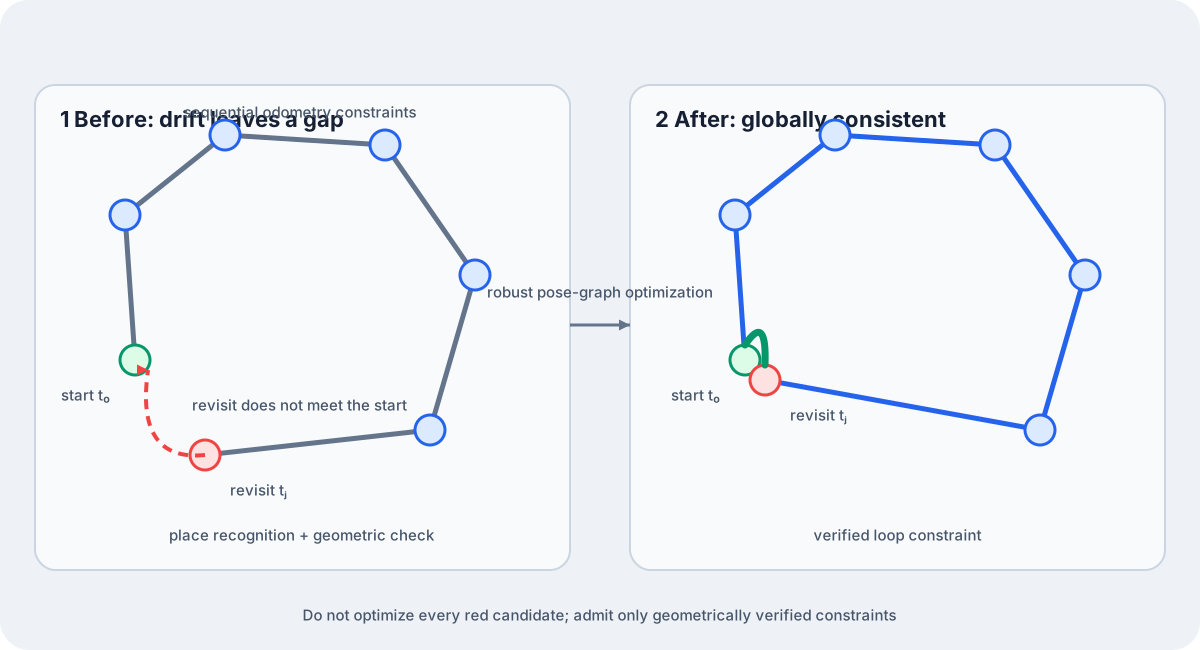
Figure 1 — Place recognition proposes a candidate, geometric verification admits a loop edge, and robust pose-graph optimization distributes accumulated drift across the trajectory. A red candidate is not accepted unconditionally.
Let the pose at time i be T_i\in SE(3), and let Z_{ij} be the relative-pose observation when time j revisits the same place. The residual of the loop constraint can be written
\mathrm{Log} is the logarithmic map that carries a rigid transform into a 6-dimensional infinitesimal rotation and translation. Combining odometry edges \mathcal E_o with loop edges \mathcal E_l, pose-graph optimization becomes
where \Omega_{ij} is the information matrix and \rho a robust loss such as Huber. Adding even a single loop edge lets error accumulated over a long trajectory be distributed across the whole graph.
2. Finding Candidates: Turning an Image into a "Bag of Words"
Bag-of-Words (BoW) quantizes local descriptors into a histogram of visual words, and computes similarity against past keyframes using inverse document frequency (IDF). ORB-SLAM-family systems pair a lightweight ORB descriptor with a vocabulary tree, narrowing candidates to a handful without comparing every frame against the whole map.
A global descriptor compresses the entire image into a single vector to retrieve similar-looking scenes. Learning-based methods like NetVLAD, CosPlace, and EigenPlaces learn representations robust to lighting and viewpoint change, but their performance shifts in buildings, farmland, or factories different from their training regions. Candidate retrieval handles speed, and geometric verification handles accuracy — you shouldn't rely on either alone.
3. Geometric Verification: Looking Similar Isn't Enough to Close the Loop
Descriptors are re-matched from the candidate image to obtain correspondences. For a monocular camera, estimate an Essential/Fundamental matrix via RANSAC; if known map points exist, use PnP; for planar texture, use a homography. Checking inlier count, reprojection error, whether depth is positive, and whether the viewpoint difference is physically plausible raises confidence that the candidate is really the same place.
A false loop is dangerous because graph optimization will warp the map into a shape consistent with — even though based on — a wrong observation. Two similar corridors, a row of windows, furrows in a field, or shelving in a factory are hard to distinguish with BoW alone. Exclude frames that are too close in time from candidates, and require consistent matches across multiple consecutive keyframes and agreement with an independent sensor (IMU/LiDAR/GNSS).
4. Updating the Pose Graph and the Map
After adding a loop edge, first optimize only the keyframe poses via the pose graph, and have the map points follow the poses. For a large-scale map, separating the local map from the global pose, rather than running Bundle Adjustment over every point every time, makes it easier to preserve real-time performance. Once optimization finishes, update the current map→odom transform, and design so that odom→base_link, which prioritizes continuity, is never made to jump suddenly.
In ROS 2 TF2 terms, local odometry publishes odom→base_link, and SLAM's global correction adjusts map→odom. Temporally smooth the correction so the robot body doesn't appear to teleport at the moment of loop closure. However, smoothing too aggressively to hide the gap between the map and the real world causes navigation to keep using a stale position, so log the correction magnitude and the time over which it's applied.
5. Environments Prone to Failure
| Condition | Why it's hard | Mitigation |
|---|---|---|
| Seasonal / day-night change | Color, shadows, vegetation change | Learned descriptors, structural features, LiDAR fusion |
| Dynamic people/vehicles | Same place, different layout | Dynamic-object masking, matching only static background |
| Repetitive patterns | Wrong places look alike too | Geometric verification, distance constraints, multi-frame confirmation |
| Long corridors/shelving | Low parallax and distinctiveness | IMU, artificial markers, UWB |
| Large lighting change | Brightness descriptors shift | HDR/exposure correction, learned place recognition |
| Sharp turns / blur | Fewer correspondences | IMU prediction, tuning keyframe interval |
6. Implementation Checklist
- Store each keyframe's image, timestamp, pose, and feature descriptors.
- Exclude recent frames from candidates, and retrieve a handful of past candidates via BoW/global descriptors.
- Geometrically verify correspondences, thresholding on inlier count, reprojection error, and positive depth.
- Confirm the same candidate holds up across multiple frames at different times.
- Add the loop edge to the pose graph and run robust optimization.
- Log the correction magnitude, rejection reasons, and compute time. Make false loops reversible.
7. Research Directions
Current research is moving in the direction of making image retrieval robust through large-scale self-supervised learning, sharing descriptors across LiDAR, camera, and event-camera modalities, and updating long-term maps seasonally. There are also attempts to use new scene representations like NeRF and 3D Gaussian Splatting for place recognition, though inference speed, memory footprint, dynamic objects, licensing, and reproducibility all need to be checked.
In factories and farmland, where identically shaped aisles or furrows repeat, image-only loop closure tends to be ambiguous. Using implement paths, IMU, wheel odometry, RTK-GNSS, and mapped work boundaries as prior knowledge to constrain the candidate search range reduces false detections. When bringing a research prototype into the field, set up from the start an operational procedure where, if a false loop is detected, the map is frozen and can be manually re-initialized.
8. Conclusion
Loop closure is a three-stage process: image retrieval that recalls a past scene, geometric verification that proves it's the same place, and optimization that distributes error across the whole graph. Don't close a loop on BoW or learned-descriptor scores alone — confirm correspondences, sensor agreement, and temporal continuity. Handled correctly, loop closure corrects odometry drift across the entire map and keeps a long-running robot's self-localization consistent.
Is a visually similar image enough to close a loop?
Appearance can produce false matches. Verify geometry before adding a constraint; a false loop can distort the entire map.
References
Current step · 16 / 19 · Computer Vision Primer
Comments
Please log in to post a comment
No comments yet.