Contents — find the section you need
Background and reading guide
Background Basic vectors, matrices and camera projection.
Fundamentals · Explanations of principles, structure and trade-offs.
Walk around holding a camera, and in the sequence of images the corner of a wall or a sign shifts a little at a time. An accelerometer and a gyroscope, meanwhile, measure at high frequency how much the device accelerated and rotated in that same interval. Visual Odometry (VO) estimates the relative pose, velocity, and position up to the present from the former; Visual-Inertial Odometry (VIO) estimates it from both. It's a core technology for drones flying indoors, AR/VR headsets, handheld 3D scanners, and mobile robots.
VO/VIO is sometimes treated as synonymous with SLAM, but the roles differ somewhat. Odometry is a front-end stage that produces a smooth, short-term relative trajectory, and its error accumulates in principle. SLAM uses a map, place recognition, and loop closure to globally correct that accumulated error. This article focuses less on the overall picture of mapping and more on how motion is integrated frame to frame, how the IMU is fused in, and when to be suspicious of the estimate.
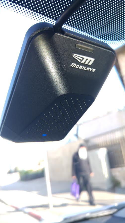 Example vehicle camera
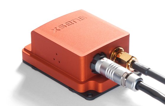 Example GNSS/INS IMU
Images: Car window camera of Mobileye system (Ranbar, CC BY-SA 4.0) / Xsens MTi-G (Kallap85, CC BY-SA 4.0), Wikimedia Commons. Representative sensors, not a required VO/VIO product combination.


0. 30-Second Summary
- VO sequentially estimates camera motion from image correspondences, or from changes in pixel appearance. Monocular VO cannot observe the absolute scale of translation, and error accumulates over time. Stereo, RGB-D, known object size, inertial sensing, and wheels all supply scale.
- VIO fuses the camera's low-frequency, drift-resistant observations with the IMU's high-frequency observations, which are accurate over short intervals but drift due to bias. The gyroscope supplies rotation; the accelerometer supplements the cue that separates gravity from acceleration.
- IMU preintegration compresses the many IMU samples between image keyframes into a single, bias-relinearizable constraint. This is what makes sliding-window optimization computationally tractable.
- Initialization is the hard part. Without sufficient parallax, excitation that includes rotation, bias estimation while stationary, and camera-IMU time synchronization and extrinsic calibration, scale, gravity, velocity, and bias cannot be disentangled.
- Evaluation should report not just the mean error but ATE/RPE, drift per interval, failure rate, latency, CPU/GPU usage, and whether the trajectory used any relocalization. Low texture, dynamic objects, motion blur, rolling shutter, shocks, and synchronization offset are the classic failure conditions.
1. What VO Estimates, and What It Doesn't
Write the pose of the camera or IMU frame B relative to the world frame W at time k as position \mathbf{p}_{WB,k} and rotation R_{WB,k}. VO's central output is the relative transform between adjacent frames or keyframes,
In feature-tracking methods, the Essential Matrix is estimated from corresponding points via RANSAC, and the rotation and translation direction are recovered from it. In stereo/RGB-D/map-based methods that already have 3D points, PnP is used on the 2D–3D correspondences. In Direct VO, rather than matching explicit descriptors, the pose is optimized so that exposure-corrected pixel values agree at their projected location.
Whichever method is used, VO is a form of dead reckoning that integrates "how far I've moved since the last frame." Without an external map or loop closure, even a tiny error in the relative pose never goes away. Position error generally grows with time and distance traveled, and even if you walk back and forth down a long corridor and return to your starting point, the trajectory won't close. This isn't just an implementation failure — it's a property of a problem that accumulates local observations sequentially.
The Monocular Scale Problem
A calibrated monocular two-view correspondence constrains E=[\mathbf{t}]_\times R, but doesn't determine the length of \mathbf{t}. That's because scaling every 3D point and translation by s>0 leaves the image projections unchanged. A monocular VO pose can look accurate while the unit of position is arbitrary — and if the scale wobbles from frame to frame, even the shape of the trajectory breaks down.
With a stereo rig of known baseline B, depth can be recovered from disparity d as Z=fB/d. RGB-D gives the sensor's own depth a fixed scale. In VIO, since acceleration is measured in units of m/s² and the magnitude of gravity is close to known, sufficient motion excitation lets you align the visual system's arbitrary scale to physical scale. But simply attaching an IMU doesn't automatically produce scale — while stationary, moving at constant velocity, over too short an interval, or with the wrong time offset, scale and bias get confused with each other.
2. Camera Observations: Feature-Based and Direct Methods
Feature-based VO uses correspondences tracked with ORB, SIFT, FAST+KLT, and similar methods. For a new frame's 2D observation \mathbf{z}_{ij} and landmark \mathbf{P}_j, the projection residual is
where \pi([X,Y,Z]^\mathsf{T})=(X/Z,Y/Z)^\mathsf{T} is the perspective division. RANSAC removes mismatches, and a Huber loss or similar keeps the remaining outliers from being over-weighted. Feature-based methods are relatively robust to exposure changes and are easier to visualize and debug geometrically.
Direct methods minimize the brightness residual of corresponding pixels or small patches. With exposure parameters a_i,b_i, the residual at a point \mathbf{u} can be written roughly as
This can exploit many textured pixels, but it's sensitive to the brightness-constancy assumption, rolling shutter, blur, auto-exposure, and reflections. Semi-direct methods take a middle ground — pixels for coarse tracking, features for the later stage.
| Method | Primary observation | Strengths | Weak conditions | Representative examples |
|---|---|---|---|---|
| Feature-based VO | Keypoint reprojection | Easy to explain, relatively robust to lighting change | Low texture, repetitive features | ORB-SLAM family, VINS-Mono |
| Direct / Semi-direct | Pixel/patch brightness | Dense information, sub-pixel tracking | Exposure change, blur, reflection | DSO, SVO |
| Monocular VIO | Image + IMU | Lightweight, scale becomes observable | Sensitive to initialization/sync | VINS-Mono, OpenVINS |
| Stereo VIO | Left/right image + IMU | Immediate scale, stable initialization | Power draw, left-right sync/calibration | VINS-Fusion, Basalt |
3. What the IMU Measures, and Why You Can't Just Integrate It Directly
An IMU outputs the gyroscope's angular velocity \tilde{\boldsymbol\omega} and the accelerometer's specific force \tilde{\mathbf{a}}. These aren't ideal values — they include bias \mathbf{b}_g,\mathbf{b}_a and white noise \mathbf{n}_g,\mathbf{n}_a.
The important point here is that the accelerometer doesn't measure world acceleration directly — it measures specific force, with gravity already subtracted out. Without knowing orientation, you don't know which direction to add gravity back in, and double-integrating even a small bias makes position drift rapidly. The continuous-time equations of motion are
Looking only at the error after one second, an IMU looks smooth and excellent, but over minutes of unaided navigation, bias and orientation error badly corrupt the position. The essence of VIO is that images correct the IMU's long-term drift, while the IMU bridges the short intervals of motion and rotation where images are sparse.
4. IMU Preintegration: Compressing Motion Between Keyframes
A typical setup runs the camera at 20–60 Hz and the IMU at 100–1000 Hz. Between keyframes i and j there can be tens to hundreds of IMU measurements. Re-integrating every sample each time the optimizer nudges the pose or bias would be expensive. Forster et al.'s IMU preintegration precomputes the relative rotation, velocity change, and position change around a given linearization-point bias, and also retains the Jacobians and covariance.
Writing the quantities with gravity and world velocity removed as \Delta R_{ij},\Delta\mathbf{v}_{ij},\Delta\mathbf{p}_{ij}, the prediction is roughly
When the bias is updated, a first-order correction is applied using the stored \partial\Delta/\partial\mathbf{b}, and full re-integration happens only when the change is large. Rotation isn't summed as a plain vector, but composed on the SO(3) manifold via the exponential map or with quaternions. Carrying a covariance \Sigma_{ij} lets a noisy IMU and a precise camera residual be weighted correctly within the same objective function.
The representative objective function for sliding-window VIO is
The state set \mathcal X includes, for every keyframe, the pose, position, velocity, gyroscope/accelerometer biases, the inverse depth of landmarks, and, where needed, the time offset or extrinsic parameters. Old states are marginalized into a prior, keeping the computational cost bounded. Because marginalization depends on the linearization point, repeatedly re-updating the state by a large amount tends to break consistency. Techniques like the First-Estimate Jacobian (FEJ) aren't just a speed optimization — they exist to keep the system from falsely "observing" degrees of freedom that are actually unobservable.
5. Filter-Based vs. Optimization-Based
VIO broadly splits into error-state extended Kalman filter (EKF) families and fixed-length nonlinear-optimization families. The former sequentially update the current state and covariance, and tend to keep latency and memory down. MSCKF doesn't keep feature points as long-lived state; instead it marginalizes them out as multi-view constraints, which keeps it lightweight. OpenVINS implements this family with an emphasis on reproducibility and extensibility.
The latter jointly optimize multiple keyframes and landmarks together. VINS-Mono is a representative example that includes feature tracking, IMU preintegration, a sliding window, and loop closure. Distributing reprojection error across multiple frames often gives an accuracy advantage, but marginalization, the solver, latency, and recovery from failed initialization all need to be designed carefully.
| Aspect | EKF/MSCKF family | Sliding-window optimization family |
|---|---|---|
| Estimation form | Sequential update of state and covariance | Iterative minimization of a factor graph over multiple timesteps |
| Compute/latency | Predictable, easy to keep low-latency | Depends on number of keyframes and iterations |
| Handling of features | Easy to marginalize as observation constraints | Easy to keep inverse depth etc. as explicit state |
| Strengths | Good for embedded, easy to handle covariance | Easier to keep reprojection broadly consistent |
| Caveats | Linearization and consistency, observability | Marginalization error, CPU load, relinearization |
Neither is universally better. Choose based on required latency, sensor frequency, CPU budget, field of view, operating environment, and maintenance capacity. Comparing only the trajectory error reported in a paper, while ignoring the camera model, calibration, dataset motion, and whether relocalization was used, is a good way to make the wrong implementation choice.
6. Initialization: What Has to Be Determined in the First Few Seconds
At the moment VIO starts, the world orientation, initial velocity, gyroscope bias, accelerometer bias, gravity, monocular scale, and camera-IMU relative pose are all undetermined. The typical flow is to build a two-view/multi-view relative structure from images alone, then align that visual motion with the IMU integration to solve for velocity, gravity direction, scale, and bias.
A stationary interval gives an initial gyroscope-bias estimate from the average gyro reading, and a cue toward gravity direction from the average acceleration direction. But an accelerometer can't distinguish a vehicle's own linear acceleration from gravity. Including "excitation" during initialization — rotating and translating along multiple axes, not just slowly moving the device back and forth — helps untangle the correlation between scale and bias. Conversely, starting with the device nearly stationary on a desk, moving at constant velocity in one direction, or seeing only a plane, tends to leave the system under-observed.
Judging initialization success isn't just about optimizer convergence. Check that the estimated scale is positive and reasonable, that the magnitude of gravity is close to about 9.81\,\mathrm{m/s^2}, that the bias isn't wildly outside the sensor's spec, and that the initial triangulated points have sufficient parallax and a high fraction of positive depth. Rather than carrying a bad old state forward after a failure, resetting the image tracks and IMU buffer and reinitializing tends to be less damaging downstream.
7. Calibration and Time Synchronization
What governs VIO's performance is less the algorithm's name than the correctness of the sensor model. At minimum, three calibrations are needed.
- Camera intrinsic calibration: focal length, principal point, distortion model. If the image is resized or cropped, K has to change too.
- Extrinsic calibration: the rigid transform T_{BC} between camera and IMU. A rotation error of a few degrees, or a lever-arm error of a few centimeters, has a large effect under fast motion.
- Time calibration: the offset between image exposure time and IMU time, and, if needed, the camera readout time. Separate clocks, buffering, and driver timestamps can leave a residual offset of several milliseconds.
Kalibr is a widely used tool for estimating the time offset and extrinsics between camera and IMU. But treating a value obtained once as permanent is risky — a focus change, reassembling the housing, temperature, or firmware time handling in the sensor can all shift these conditions. Rather than just copying typical values from a datasheet, checking the IMU noise density and bias random walk with something like Allan variance helps avoid over-trusting the filter.
A rolling-shutter camera doesn't capture a single frame at one instant. Under fast rotation, the top and bottom rows are observed at different poses, and a reprojection residual that assumes a global shutter will be systematically off. A short exposure with a global shutter is the most reliable fix; failing that, consider an observation model that includes row timing, together with IMU compensation. When adding left/right cameras or a depth sensor, hardware-triggered synchronization is preferable.
8. Choosing an Implementation: VINS-Mono, OpenVINS, and Related Systems
VINS-Mono is a widely referenced optimization-based VIO implementation for a monocular camera plus IMU. It includes online extrinsic and time-offset calibration, feature tracking, preintegration, a sliding window, and loop closure. Its value isn't just outputting a pose — it's that the whole configuration is legible for research purposes. VINS-Fusion is a candidate when you want to combine stereo or GPS.
OpenVINS is an open implementation centered on the MSCKF/EKF family, designed with FEJ and consistency made explicit. It suits situations where you want to verify how a filter-based VIO handles state, covariance, and calibration. Basalt provides stereo VIO with a high-performance optimization backend and is exercised against datasets like EuRoC. On smartphones and in AR, using the platform's built-in VIO is often more realistic for an application, since it has access to camera timing, IMU timing, and device-specific calibration.
| Implementation/family | Estimation style | Example sensor config | Suited for | Things to check when adopting |
|---|---|---|---|---|
| VINS-Mono | Optimization, fixed window | Monocular + IMU | Learning the overall structure of VIO, research prototyping | ROS generation, calibration format, initialization conditions |
| VINS-Fusion | Optimization, fixed window | Monocular/stereo + IMU, GPS optional | Multi-sensor prototyping | Coordinate frames and weighting of absolute observations |
| OpenVINS | EKF/MSCKF | Monocular/stereo + IMU | Embedded-leaning, filter verification | Noise values, FEJ, state design |
| Basalt | Optimization | Stereo + IMU | High-performance VIO backend | Build environment, camera model |
| Custom OpenCV + Ceres | Arbitrary | Arbitrary | Requirement-specific work, learning | Verifying reprojection, preintegration, marginalization |
When comparing existing implementations, don't treat a trajectory showing up in a demo as success. Verify on real hardware: the input image's resolution and actual frequency, the IMU's units and axis convention, the time reference, extrinsic calibration, behavior on initialization failure, relocalization after tracking loss, CPU usage, memory, and license. In particular, if a ROS message's timestamp gets filled in with "receipt time," the estimator receives an order that looks correct but time intervals that are physically wrong.
9. A Minimal Processing Flow
- Calibrate camera intrinsics/extrinsics and time, and buffer images and IMU data on a common time base.
- On each IMU arrival, predict the state using bias-corrected angular velocity and specific force, and update the covariance or preintegration.
- On each image arrival, track features from the previous frame/keyframe, and remove outliers with forward-backward checks, RANSAC, and masks.
- Before initialization, judge parallax and excitation, and align visual structure with inertial data. Delay the start if conditions are poor.
- After initialization, fuse the visual reprojection residual with the IMU residual, updating pose, position, velocity, bias, and points.
- Marginalize old keyframes, and discard observations that fail a quality gate. Transition to relocalization or a safe reset if needed.
In this flow, the distinction between predict and correct matters. Even if images are temporarily lost, IMU prediction can keep producing output, but its uncertainty is growing. Rather than a binary "pose available / not available," the application side should receive tracking state, a covariance or quality score, and time since the last visual update, and use them to progressively switch AR display, control velocity, and safety stops.
10. Evaluation Metrics: What to Measure to Compare Fairly
Absolute Trajectory Error (ATE) is the difference between the estimated position sequence and ground truth after aligning them with a rigid or Sim(3) transform.
Since monocular VO has undetermined scale, always state whether the Sim(3) alignment also matched the scale. If you actually want to see the scale error in VIO or stereo, Sim(3) alignment will hide exactly that error. Whether to use an SE(3) alignment, align only the starting pose, or compare trajectories unaligned should be chosen according to the purpose.
Relative Pose Error (RPE) measures local drift over a fixed time or distance interval \Delta. From the difference between the estimated relative transform \hat T_{k,k+\Delta} and ground truth T^{\mathrm{gt}}_{k,k+\Delta},
translation error (m/m or %) and rotation error (deg/m, deg/s) are computed. Even if ATE over a long distance is small, a trajectory unsuitable for AR or flight control if short-term jitter is large. Conversely, a trajectory that's smooth but drifts over long distances is unfavorable for mapping.
| Metric | What it mainly tells you | Pitfall |
|---|---|---|
| ATE RMSE/median | Overall positional consistency of the trajectory | Value changes a lot depending on alignment method |
| RPE (distance/time interval) | Local drift, effect on control | Not comparable unless the interval length is stated |
| Rotation error | Quality of gyroscope/visual orientation | Mixing yaw with roll/pitch hides the cause |
| Scale error | Physical scale of monocular VIO/stereo | Cannot be evaluated after Sim(3) alignment |
| Track rate / failure rate | Real-world availability | Don't hide automatic reinitialization after failure |
| Latency / CPU / power | Practicality of an embedded implementation | Can't be judged from offline processing alone |
EuRoC MAV, TUM VI, UZH-FPV, and KITTI are public datasets commonly used for comparison. But indoor handheld cameras, vehicle-mounted setups, and racing drones differ in field of view, lighting, speed, vibration, and exposure. Rather than importing a benchmark ranking directly onto real hardware, evaluate on a route, speed, and failure condition close to your own logs. Even in the field where ground truth can't be captured, you can audit against the start/end gap of a closed loop, known distances, wall reprojection, or a partial section covered by external motion capture.
11. Representative Failure Conditions and Countermeasures
Low texture, darkness, blur
A white wall, a dark corridor, backlighting, or a sharp turn leave insufficient gradient in the visual residual. Loosening the RANSAC threshold when there are few feature points just increases mismatches. Countermeasures include lighting/sensor design that shortens exposure time, going wide-angle or stereo, re-detecting features, and notifying the consumer of increased predicted uncertainty.
Dynamic objects and reflections
VIO assumes that most image points belong to the static background. Crowds, a lead vehicle in traffic, mirrors, glass, and water surfaces all break that assumption. Robust loss and RANSAC alone can't save a case where the background ends up a minority. What's needed is excluding the semantic region of moving objects, separating multiple motions with depth or flow, and a design that prioritizes fixed objects.
IMU saturation, vibration, temperature drift
Motor vibration in drones and small robots injects strong band-limited noise into the accelerometer, and shocks can saturate its range. Setting the filter's noise too small and over-trusting the IMU makes it reject image corrections and diverge. Use vibration isolation, appropriate band-limiting, saturation flags, a bias model that includes temperature, and measured noise parameters. Also be careful — over-smoothing the raw IMU loses short accelerations.
Time offset and coordinate-frame mix-ups
A 5 ms time offset corresponds to a large field-of-view difference during fast rotation. Be explicit about whether image timestamps mean exposure start, exposure midpoint, or receipt time, and whether IMU timestamps mean sample time or arrival time. Mixing up right-handed/left-handed conventions, the sign of gravity, T_{BC} versus T_{CB}, or the direction of the camera's optical axis can leave the optimization numerically converged but physically wrong. Prepare unit tests using a stationary test, a known 90-degree rotation, and a short straight-line move.
Confusing initialization with relocalization
Initialization is starting an estimate from a state with no map or scale yet; relocalization is returning to a known map or a past keyframe. Pure VO/VIO typically restarts in a new local coordinate frame whenever tracking is lost. Don't confuse the relocalization capability of loop-closing SLAM with VO's raw drift performance when evaluating. In a product, explicitly decide whether to keep using the old coordinate frame after tracking loss, stop safely, or invalidate the anchor.
12. Recent Directions
In recent years, learning-based feature and correspondence estimation such as SuperPoint, LightGlue, and LoFTR has, in some cases, proven effective against appearance changes that are hard for classical local descriptors. Approaches that combine a deep network with iterative geometric optimization, such as DROID-SLAM, have also appeared. But even when a learned model returns many correspondences, scale ambiguity, planar degeneracy, time synchronization, and IMU bias remain physical problems. A design that verifies learned output against robust geometry, reprojection error, and inertial consistency is still the fundamental approach.
Event cameras, with their high speed and high dynamic range, have the potential to cover conditions where a conventional camera struggles with blur or darkness. Multi-modal estimation that adds LiDAR, UWB, GNSS, or wheel odometry into VIO is also becoming practical, as a countermeasure for long-term drift and harsh environments. Adding more sensors doesn't automatically improve performance — extrinsics, timing, fault detection, and weight tuning all become new potential failure surfaces.
13. Summary
VO is a useful odometry technique for recovering short-term relative motion from images, but monocular VO has no scale and local error accumulates. VIO combines the IMU's high-frequency motion constraint with the camera's long-term correction, simultaneously estimating scale, pose, velocity, and bias. Its core is a correct sensor model, IMU preintegration, initialization using sufficient motion excitation, and a robust fusion of visual and inertial residuals.
In practice, first verify calibration, timing, and coordinate frames, then turn parallax, inlier distribution, reprojection error, bias, gravity, and tracking state into observable logs. VINS-Mono and OpenVINS are strong starting points, but need to be evaluated against your capture conditions, latency, reinitialization policy, and safety requirements. What should ultimately be trusted isn't how good the trajectory looks, but a design that can explain under which conditions scale and pose are observable, and under which conditions uncertainty grows.
Does adding an IMU always stabilize scale?
Observability depends on motion. Insufficient excitation or calibration error can leave estimation unstable despite the extra sensor.
References (Primary Sources and Official Documentation)
- Scaramuzza & Fraundorfer, Visual Odometry: Part I (IEEE Robotics & Automation Magazine, 2011)
- Forster et al., On-Manifold Preintegration for Real-Time Visual-Inertial Odometry (IEEE TRO, 2017)
- Qin, Li & Shen, VINS-Mono: A Robust and Versatile Monocular Visual-Inertial State Estimator (IEEE TRO, 2018)
- Geneva et al., OpenVINS: A Research Platform for Visual-Inertial Estimation (ICRA 2020)
- OpenVINS Official Documentation
- VINS-Mono Official Repository
- Kalibr Official Repository
- EuRoC MAV Dataset (ETH Zurich)
- TUM VI Benchmark
- DROID-SLAM paper (NeurIPS 2021)
Current step · 15 / 19 · Computer Vision Primer
Comments
Please log in to post a comment
No comments yet.