Contents — find the section you need
Background and reading guide
Background Basic frames, velocity and sensor terminology; use the reading guide for background.
Fundamentals · Explanations of principles, structure and trade-offs.
Neither Visual-SLAM nor LiDAR-SLAM works everywhere on its own. A camera struggles in the dark or under fast motion; LiDAR struggles in feature-poor environments and costs more. The key to covering these weaknesses is the IMU (Inertial Measurement Unit), which measures acceleration and angular velocity at high frequency. VIO (Visual-Inertial Odometry) and LIO (LiDAR-Inertial Odometry) -- pairing a camera or a LiDAR with an IMU -- have become the de facto standard configuration in a great many autonomous mobile robots, drones, and AR/VR devices today. This article starts from the principle behind why an IMU alone cannot sustain a position estimate, works through the idea of sensor fusion, the two design philosophies of Filter-based and Optimization-based estimation, and finally the landmark algorithms: ROVIO, OKVIS, VINS-Mono, OpenVINS, LIO-SAM, and FAST-LIO2.
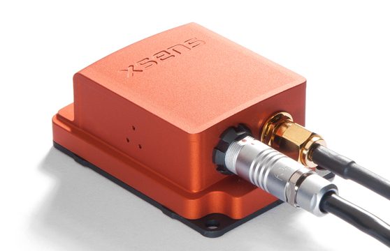 IMU/INS example
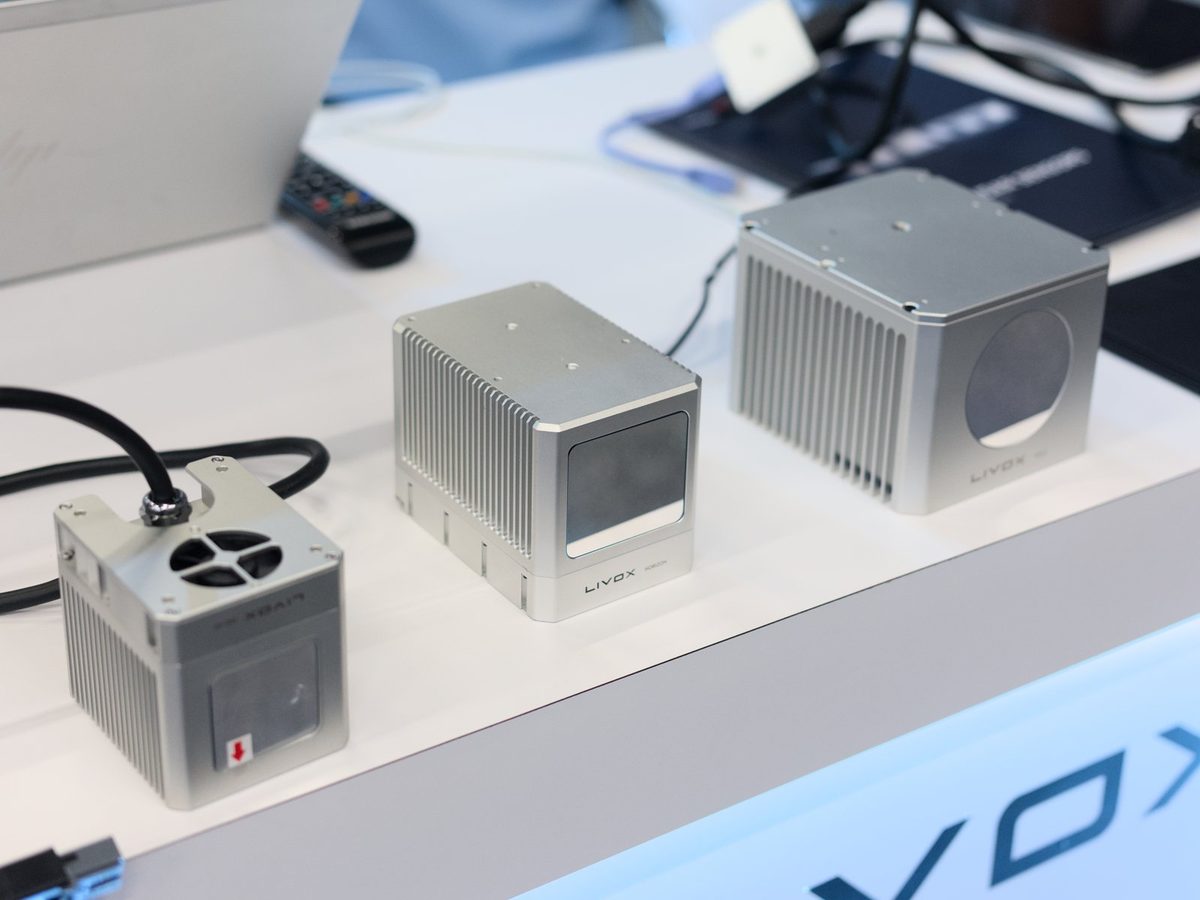 LiDAR example
Images: Xsens MTi-G (Kallap85, CC BY-SA 4.0) / Livox Mid-40, Horizon, and Tele-15 (Dllu, CC BY-SA 4.0), Wikimedia Commons. Representative input sensors, not a required VIO/LIO hardware configuration.


0. What This Article Covers
- What an IMU measures, and why an IMU alone cannot keep recovering position over time
- The weaknesses of a Camera and a LiDAR respectively, and why combining either with an IMU works so well
- What VIO and LIO each refer to, and how they differ
- The difference between the Filter-based (EKF/MSCKF) and Optimization-based (Factor Graph) design philosophies
- What ROVIO, OKVIS, VINS-Mono, VINS-Fusion, and OpenVINS (VIO) and LIO-SAM, FAST-LIO, and FAST-LIO2 (LIO) each contribute
- How to actually choose between VIO and LIO in practice, by use case
1. The Short Answer: What an IMU, VIO, and LIO Are
In one sentence each: An IMU (Inertial Measurement Unit) is a sensor that combines an accelerometer and a gyroscope to measure its own acceleration and angular velocity at high frequency, with no reference to any external landmark whatsoever. VIO (Visual-Inertial Odometry) is the technique of combining this IMU with a camera to estimate self-position and orientation; LIO (LiDAR-Inertial Odometry) does the same by combining an IMU with a LiDAR.
An IMU tells you, at high frequency (typically hundreds of Hz up to around 1 kHz), "how hard am I accelerating and how fast am I rotating, right now" -- but its integrated quantity, position, drifts away rapidly over time (we look at this closely in Section 3). A camera or a LiDAR, by cross-referencing the surrounding environment, can supply relative position constraints, but only at low frequency (tens of Hz), and both lose function entirely in certain situations -- darkness, feature-poor scenes, fast motion. The core idea of VIO and LIO is to combine this "high-frequency but drifting IMU" with a "low-frequency Camera/LiDAR that has environment-dependent failure modes," so that each covers for the other's weakness.
2. What Does an IMU Actually Measure?
Inside an IMU there are, broadly, two kinds of sensors.
An accelerometer measures specific force in its sensor frame. Ideally, \mathbf{f}_b=R_{wb}^{T}(\mathbf{a}_w-\mathbf{g}_w), where R_{wb} rotates sensor coordinates into world coordinates, \mathbf{a}_w is world-frame acceleration, and \mathbf{g}_w is gravity. It reads about 1 g at rest and nearly zero in ideal free fall. Before integration, correct bias, rotate into the world frame, and add gravity. See the coordinate and bias definitions in the OpenVINS IMU model.
A Gyroscope measures the sensor's own rate of rotation, i.e. angular velocity. Combining three axes here simultaneously gives the rotation rate around roll, pitch, and yaw.
By combining these two kinds of sensors, an IMU can output 6-degree-of-freedom motion information (3 translational + 3 rotational) at high frequency, purely from the sensor's own internal state, with no reference to any external landmark (a mapped feature, a radio signal) whatsoever. This "no external reference at all" property is simultaneously the IMU's greatest strength and its greatest weakness -- the strength is robustness that holds up unchanged in total darkness or inside a glass-walled room; the weakness is the accumulating error we look at in Section 3.
An IMU's output also always contains Bias and Noise. Bias is an offset error intrinsic to the sensor -- the output isn't zero even when the true value is zero -- and it drifts slowly over time due to factors like temperature change (Bias Instability). Noise is a random fluctuation added anew with every reading. Cheaper MEMS (Micro-Electro-Mechanical Systems) IMUs tend to have larger bias and noise, and this is the primary cause of the Drift discussed next.
3. Finding Position from an IMU Alone (Integration and Drift)
Recovering position from IMU output requires integrating acceleration twice: velocity is the integral of acceleration, and position is the integral of velocity.
Here p_0 is the initial position, v_0 the initial velocity, and a(s) the acceleration at time s. The formula itself is simple, but the acceleration a(s) actually used in practice always carries the bias b discussed in Section 2. Double-integrating an acceleration that includes bias, a(s) + b, produces a bias-driven error term of the form
which diverges in proportion to the square of elapsed time. Gyroscope bias, on top of this, gradually skews the orientation estimate, and that orientation error contaminates the direction in which acceleration gets integrated -- so overall position error tends to grow on the order of O(t^2) to O(t^3). This phenomenon, where error accumulates without bound over time, is called Drift.
A concrete number helps build intuition here. Suppose a cheap MEMS IMU has an accelerometer bias of roughly 0.01\,\mathrm{m/s^2}. After 10 seconds, the resulting position error is about \frac{1}{2} \times 0.01 \times 10^2 = 0.5\,\mathrm{m}. After a minute, the number works out to 18\,\mathrm{m}. An IMU alone can only be trusted for a position estimate over a very short time scale -- seconds to a few tens of seconds -- and this is the fundamental reason an IMU alone cannot serve as a self-localization system. Put the other way around: an IMU is strong at "short-term, high-frequency change" and weak at "long-term, absolute position" -- exactly the opposite profile of strengths and weaknesses from a Camera or LiDAR.
4. A Camera and a LiDAR Have Weaknesses Too
If an IMU alone can't recover position, the obvious thought is to just use a Camera (see "Visual-SLAM Primer") or a LiDAR (see "LiDAR-SLAM Technology Trends") instead. That's true as far as it goes, but a Camera and a LiDAR each carry their own distinct weaknesses.
A Camera's weaknesses are image degradation in low light (feature points, or the brightness gradients a Direct method relies on, become impossible to compute), low-texture environments (a plain white wall or a solid-colored floor yields no correspondence points at all), and Motion Blur under fast movement (the image smears during the exposure window, destabilizing feature descriptors). All of these share the same underlying cause: the camera isn't getting enough visual signal to work with.
A LiDAR's weaknesses are feature-poor environments (in a long tunnel or a wide-open plane, point-cloud registration methods like ICP/NDT can't converge to a unique solution -- what's called geometric degeneracy) and the sensor's cost. LiDAR actively emits a laser to measure range, so it's robust to darkness and backlighting, but in a place where the environment's own geometry is sparse, it loses its footing in much the same way a camera does.
An IMU's weakness, as seen in Section 3, is the unbounded Drift that accumulates over time, and the fact that it has no means, on its own, of recovering absolute position at all.
The important point is that the situations in which these three sensors fail barely overlap at all. An IMU keeps working unfazed in the darkness where a Camera struggles, and it keeps supplying high-frequency motion information right through the moment a Camera or LiDAR loses its features. Camera and LiDAR observations constrain drift using environmental geometry. They do not guarantee long-term absolute position accuracy without constraints such as a known map, GNSS, or loop closure. This complementarity is the starting point for the sensor fusion discussed in the next section.
5. The Idea of Sensor Fusion
Sensor Fusion is the framework of combining several sensors' distinct error characteristics and areas of strength to obtain an estimate that is more accurate, higher-frequency, and more robust than any single sensor alone (for the general idea of fusion, see "Sensor Fusion Primer"). The skeleton shared by VIO and LIO can be organized as a Predict-Update loop:
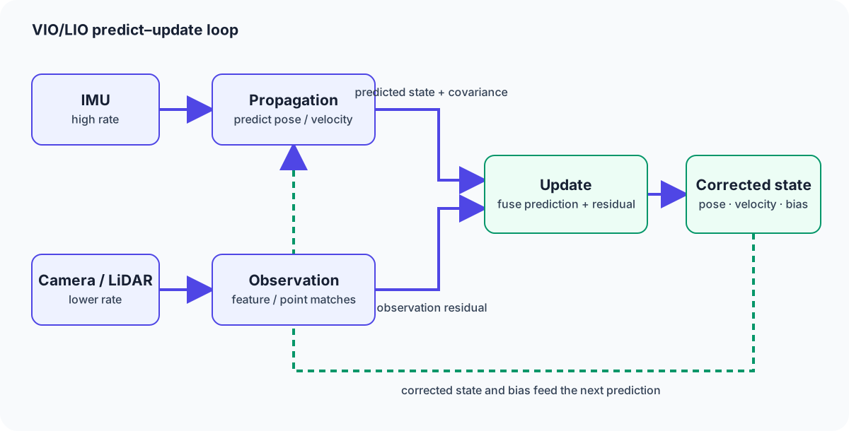
Figure 1 — The IMU (high-rate) keeps predicting state via Propagation (integration). Observations from feature/point matching against the Camera/LiDAR (low-rate) correct that prediction in the Update step. The IMU bias estimated during that correction is fed back into the next Propagation, continuously suppressing Drift accumulation.
This loop has two key points. First, IMU-driven Propagation runs at high frequency continuously, and never stops predicting pose even in the moments when no Camera/LiDAR observation is available (darkness, low texture, feature-poor space, fast motion). Second, the Update step -- which only fires when a Camera/LiDAR observation arrives -- reduces the Drift that would otherwise accumulate without bound from the IMU alone, and simultaneously updates the estimate of the IMU's own bias, feeding it back into Propagation. This combination -- "prediction that keeps running at high frequency" plus "correction that reduces errors in directions constrained by the observation" -- is the design philosophy shared by VIO and LIO.
6. VIO (Visual-Inertial Odometry)
VIO (Visual-Inertial Odometry) is the configuration in which a Camera plays the Update-side sensor role within this framework. Combining the IMU's high-frequency prediction with a Camera's feature-point observations resolves the scale ambiguity that plagues monocular Visual Odometry (touched on in Section 4 -- the fact that monocular images alone cannot recover a real-world, metric distance), using the IMU's metric acceleration information. And in fast motion, where a Camera struggles, the IMU keeps supplying orientation change at high frequency throughout, making tracking far less likely to fail outright.
VIO further splits into Loosely-Coupled and Tightly-Coupled configurations, depending on how the Camera and the IMU are tied together. A loosely-coupled system computes the Camera-side pose estimate and the IMU-side pose estimate independently and then fuses the two results after the fact; it's simple to implement, but because the IMU side can't exploit the internal error structure of the Camera-side estimate (which feature observation is more or less uncertain), it loses out on precision. A tightly-coupled system treats the IMU's raw data and the image's feature observations as a single, jointly estimated state problem from the outset; implementation is more complex, but every bit of information from both sensors gets used, yielding higher precision. The representative modern VIO implementations we cover in Sections 8, 9, and 10 (OKVIS, VINS-Mono, OpenVINS, and others) all adopt tight coupling.
7. LIO (LiDAR-Inertial Odometry)
LIO (LiDAR-Inertial Odometry) is the same framework with a LiDAR playing the Update-side role. LiDAR point clouds capture environmental geometry directly and with high precision, but a single scan takes tens to hundreds of milliseconds to sweep, and if the sensor itself moves during that window, the resulting point cloud distorts (Motion Distortion). With the IMU's high-frequency orientation information on hand, this in-scan motion can be corrected, reconstructing a distortion-free point cloud.
As with VIO in Section 6, in geometrically degenerate environments that LIO struggles with (long tunnels, wide-open planes), the IMU's continued short-term pose prediction makes point-cloud registration (methods like ICP/NDT) far less likely to diverge. LIO, too, is predominantly implemented as a tightly-coupled system in practice -- LIO-SAM and FAST-LIO/FAST-LIO2, covered in Section 10, both adopt this tightly-coupled design.
8. Filter-based (Kalman Filter / EKF / MSCKF)
The core of VIO and LIO -- fusing prediction and observation -- is implemented under one of two broad design philosophies: Filter-based, or the Optimization-based approach covered in the next section.
The foundation of the Filter-based approach is the Kalman Filter, a framework that alternates Prediction and observation-driven Update to recursively derive the optimal state estimate for a system with linear dynamics. For a problem like VIO/LIO, where the composition of IMU integration (pose composition) and the Camera's projection are inherently nonlinear, the nonlinear extension is used instead: the EKF (Extended Kalman Filter). An EKF linearizes each nonlinear function around the current estimate (a first-order Taylor expansion) and then applies the same update equations as an ordinary Kalman Filter.
Here \hat{x}_k^{-} is the predicted state from Propagation, z_k the actual observation, h(\cdot) the observation model that predicts an observation from the state, and K_k the Kalman Gain -- the weight that decides how much to trust the prediction versus the observation. P_k^{-} is the covariance (uncertainty) of the predicted state, H_k the Jacobian linearizing the observation model, and R the covariance of observation noise. Intuitively, the larger the predicted uncertainty P_k^{-} is relative to the observation noise R, the larger the Kalman Gain K_k becomes, and the more strongly the observation z_k's information gets folded into the state correction.
Implementing an EKF-based VIO naively requires including every individual feature point from the image in the state vector, and computational cost balloons rapidly as the number of feature points grows. The MSCKF (Multi-State Constraint Kalman Filter), proposed by Mourikis & Roumeliotis in 2007, solves exactly this problem. MSCKF does not include feature points themselves in the filter's state; instead it keeps multiple camera poses (a sliding window) in the state, and updates the state using only the geometric constraint that the same feature point was observed from several of those poses. By excluding feature points from the state, it avoids the computational blowup with feature count while still exploiting observations spanning multiple frames -- an efficient Filter-based VIO design that's now in wide use.
9. Optimization-based (Bundle Adjustment / Factor Graph)
Filter-based estimation updates recursively, but methods such as MSCKF can temporarily retain cloned past poses. The Optimization-based approach keeps state and observations spanning a sliding window or graph and solves a nonlinear optimization for their joint consistency. It helps to think of it as extending Visual-SLAM's Bundle Adjustment (see "Visual-SLAM Primer", Section 10) to also incorporate IMU information.
IMU accelerations and angular rates are known observations, not optimization variables. Adding a state at every IMU timestamp, or reintegrating every interval at each relinearization, increases cost. IMU Preintegration, proposed by Forster et al. in 2015 (arXiv:1512.02363), summarizes measurements between keyframes as a bias-correctable relative-motion factor. The state can include velocity and biases, and in some systems landmarks as well; cost is controlled by window design and relinearization rather than simply by the IMU sample rate.
The resulting IMU Preintegration Factor, together with Factors derived from Camera/LiDAR observations (reprojection error or scan-matching error), are placed on a common Factor Graph, and the whole thing is solved together as a maximum-likelihood (or maximum a posteriori) estimation problem -- this is the basic form of the Optimization-based approach.
\mathcal{X} is the set of poses, velocities, biases, and (where needed) map points to be estimated; r_{\mathrm{IMU}} is the residual from the preintegration factor. Filter-based estimation controls cost through sequential updates and bounded history; optimization-based estimation can relinearize a sliding window. Accuracy and cost depend on window length, initialization, relinearization schedule, model, and compute budget, so neither is universally superior.
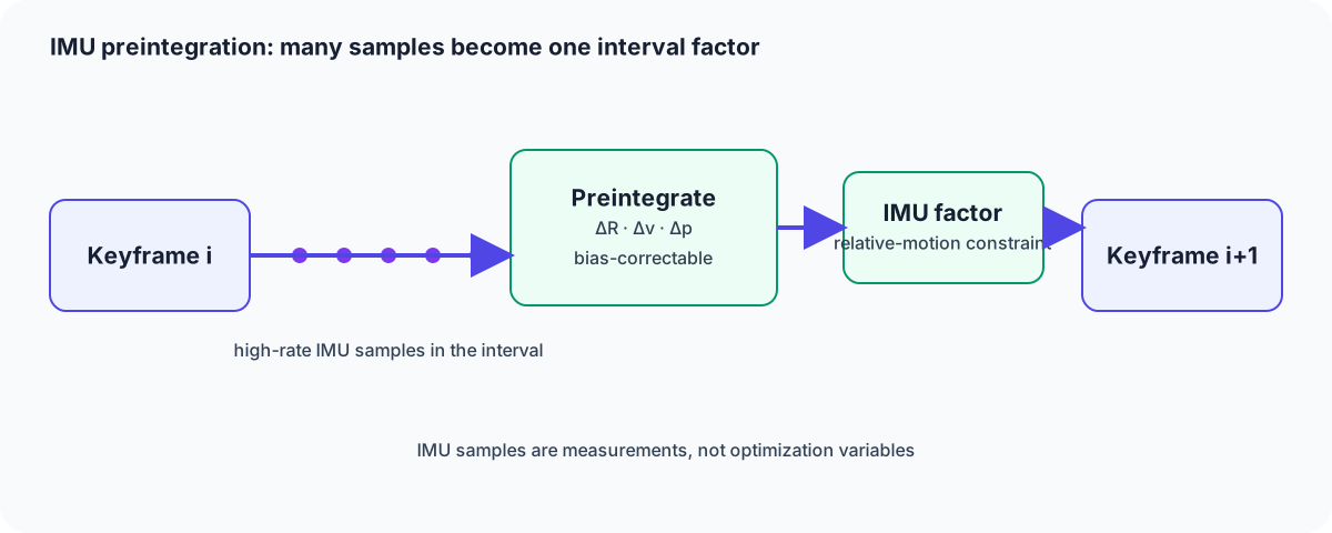
Figure 2 — The large number of IMU measurements (hundreds of Hz) arriving between Keyframe i and i{+}1 are integrated together in advance via Preintegration, and handled on the Factor Graph as a single relative-motion Factor. This keeps the number of optimization variables independent of the IMU's sampling rate -- dependent only on the number of keyframes.
10. Landmark Algorithms
VIO
ROVIO (Robust Visual Inertial Odometry), presented by Bloesch et al. at IROS 2015, is an EKF-based VIO. Rather than matching feature-point descriptors, it feeds image-patch brightness information directly into the EKF's observation model -- a Direct-method-style approach that makes it a representative example of combining Filter-based estimation with a Direct method.
OKVIS (Open Keyframe-based Visual-Inertial SLAM), presented by Leutenegger et al. in IJRR 2015, is a keyframe-based VIO built on nonlinear optimization. Combining IMU Preintegration (Section 9) with Bundle-Adjustment-style reprojection error minimization, it is one of the earlier landmark implementations of Optimization-based VIO.
VINS-Mono, from Qin, Li, and Shen at the Hong Kong University of Science and Technology, is a VIO for monocular cameras that builds on nonlinear optimization over IMU Preintegration (Section 9), adds Loop Closure for global correction, and offers a flexible design that can be switched between loosely- and tightly-coupled operation for each component. VINS-Fusion is the successor that extends VINS-Mono to support multiple sensor configurations -- stereo cameras, GPS -- prioritizing practicality across more diverse hardware setups.
OpenVINS, from Geneva, Eckenhoff, Lee, Yang, Huang, and collaborators, is an open-source MSCKF-based VIO research platform. Building on the efficient Filter-based design of MSCKF (Section 8), it's widely used as an implementation that prioritizes ease of extension and validation for research purposes.
LIO
LIO-SAM (Tightly-coupled Lidar Inertial Odometry via Smoothing and Mapping), presented by Shan, Englot, Meyers, Wang, Ratti, Rus, and collaborators at IROS 2020, is a tightly-coupled LIO built on a Factor Graph. It unifies several Factor types -- an IMU Preintegration Factor, an Odometry Factor from LiDAR scan matching, a GPS Factor, and a Loop Closure Factor -- on the same Factor Graph, and is a representative example of applying the Optimization-based design philosophy (Section 9) to LiDAR.
FAST-LIO (Fast LiDAR-Inertial Odometry), from Xu, Zhang, and collaborators at the University of Hong Kong's MARS Lab, is a fast LIO built on a Tightly-Coupled Iterated Kalman Filter. In contrast to the Optimization-based LIO-SAM, it's Filter-based, designed to handle high-rate LiDAR point clouds directly, and prioritizes real-time operation on platforms with limited compute. FAST-LIO2 is its successor: by managing the point cloud directly with an incremental nearest-neighbor search structure (an iKD-Tree), it dramatically cuts the cost of rebuilding the map, achieving a faster and more accurate tightly-coupled LIO.
11. VIO vs. LIO Comparison
| Aspect | VIO (representative: VINS-Mono/OpenVINS) | LIO (representative: LIO-SAM/FAST-LIO2) |
|---|---|---|
| Primary sensor | Camera (mono/stereo) + IMU | LiDAR + IMU |
| Environments it favors | Indoor/outdoor scenes rich in texture, where color and pattern recognition carries meaning | Environments rich in geometric structure; works in darkness or backlighting |
| Environments it struggles with | Darkness, low texture, backlighting/strong sunlight | Geometrically degenerate spaces -- long tunnels, wide-open planes |
| Sensor cost | Relatively low (camera + MEMS IMU) | High (the LiDAR unit itself, especially long-range, high-resolution models) |
| Map character | Sparse feature points, or dense depth with a learning-based approach | Dense, geometrically accurate point-cloud map |
| Scale ambiguity | Present in principle for a monocular configuration (resolved via the IMU) | Not present in principle, since LiDAR ranging is inherently metric |
| Compute | Moderate (cost of feature extraction and descriptor computation) | Point-cloud processing (nearest-neighbor search, scan matching) carries a comparable cost |
| Representative design philosophy | Both Filter-based (MSCKF) and Optimization-based (Preintegration + BA) are widely deployed | Both Filter-based (FAST-LIO2) and Optimization-based (LIO-SAM) are widely deployed |
VIO's strengths are its low sensor cost and the high-level environmental understanding that color and pattern recognition affords (a natural fit with object recognition); LIO's strengths are geometric accuracy and robustness to darkness and bad weather -- that's the basic division of labor.
12. Choosing One in Practice
Whether to choose VIO, LIO, or a combination of both depends on the sensors you can carry, your budget, and the environment you expect to operate in.
- Indoor service robots / robot vacuums: If low cost is the priority, VIO (or a loosely-coupled camera-plus-IMU configuration) tends to win out; if precision and a geometrically accurate map are the priority, LIO tends to be chosen. In a regular indoor environment with lots of corridors and walls, the accuracy gain from LiDAR's cost is easier to justify.
- Drones: With tight constraints on payload and power, a lightweight camera-plus-IMU VIO configuration tends to dominate. In open outdoor spaces, pairing with GPS is also common.
- AR/VR: A VIO (Visual-Inertial Odometry) using the headset's built-in camera and IMU is the de facto standard; barring a few high-end models with an added LiDAR, cost and weight constraints make VIO the default first choice.
- Autonomous driving / outdoor autonomous mobile robots: Given the demand for robustness in bad weather, backlighting, and nighttime driving, LIO is typically the backbone, layered together with VIO and GNSS (see "Sensor Fusion Primer").
- Geometrically degenerate spaces -- tunnels, long straight corridors: LiDAR alone, or LIO alone, tends to become unstable in registration, so it's important to add a separate information source -- VIO, or wheel odometry -- to cover for the degeneracy.
The basic rule of thumb: if budget and sensor weight allow and geometric precision is the top priority, choose LIO; if cost and light weight are the priority and you also want to exploit color/pattern-based environmental understanding, choose VIO. In actual product development, the two are rarely chosen exclusively -- instead, they tend to evolve into a multi-sensor fusion (see "Sensor Fusion Primer") that weights VIO, LIO, GNSS, and wheel odometry according to the situation.
13. Summary
An IMU delivers high-frequency, fully self-contained motion information, but position recovered by integration Drifts rapidly, on the order of the square to the cube of elapsed time. A Camera (VIO) or a LiDAR (LIO) periodically corrects this accumulated error, but each carries its own separate weakness -- darkness and low texture for the Camera, geometrically degenerate environments for the LiDAR. VIO and LIO combine these complementary weaknesses through a Predict (high-frequency IMU prediction) - Update (Camera/LiDAR correction) loop, implemented under either the Filter-based (EKF/MSCKF) or Optimization-based (IMU Preintegration + Factor Graph) framework, to achieve a robustness and precision that no single sensor can reach alone.
Should the roughly 1 g reading at rest be integrated directly?
Transform specific force into the world frame and account for gravity and bias first. Growing velocity at rest signals a model or frame problem.
Current step · 10 / 18 · Robotics Primer
Comments
Please log in to post a comment
No comments yet.