Contents — find the section you need
Background and reading guide
Background Basic functions, calculus and vectors; follow the definitions alongside the equations.
Fundamentals · Explanations of principles, structure and trade-offs.
A robot rarely reads the state it needs directly. An encoder may expose position but not velocity; an IMU reports acceleration and angular rate with bias; camera localization arrives late or disappears. A state observer uses a plant model and the gap between predicted and measured output to estimate hidden state. The linear Kalman filter (KF) is the standard observer that carries an error covariance and uses assumed process and measurement noise to decide how much to trust prediction versus measurement.
The key idea is not “average sensors.” It is to state which physical time a datum represents, what error model is assumed, and what happens when sensors disagree. An estimator that is confidently wrong drives PID, LQR, and MPC toward the wrong place. For ROS 2 timing and execution boundaries, read ROS 2 Primer; for broader sensor integration, read Sensor Fusion Primer.
Practical conclusion
- An observer updates \hat{x} from model prediction and innovation. An unobservable state cannot be uniquely reconstructed merely by selecting a smarter filter.
- KF carries state-error covariance P and uses process covariance Q and measurement covariance R to calculate the Kalman gain K.
- Q,R are assumptions about model and sensor errors, not arbitrary “accuracy knobs.” Validate them with innovations, covariance, timestamps, and fault data.
- If an estimate is stale, covariance is excessive, innovation is anomalous, or transforms fail, pass a degraded state to control and reduce or stop motion according to the hazard.
State-space observer and observability
For a discrete linear system,
x is true state, u known input, z measurement, w process disturbance, and v measurement noise. A Luenberger observer has the form
The final term is the innovation. A high observer gain L follows measurement quickly but transmits more noise; a low L trusts the model longer but corrects disturbances slowly.
Diagram: Duskcoil, conceptual rather than measured. Estimate and covariance are internal model quantities, not direct sensor observations.
The observability matrix \mathcal O=[C^T,(CA)^T,\ldots]^T must have full rank to reconstruct every state in the ideal linear case. Position-only measurements of a double integrator can make velocity observable through time history, but sampling rate, quantization, delay, and dropout determine whether the resulting estimate is useful. “Observable” is not a substitute for a maximum latency and accuracy requirement.
Kalman prediction and update
Assuming zero-mean white Gaussian w\sim\mathcal N(0,Q) and v\sim\mathcal N(0,R), the prior is
P is uncertainty of estimation error, not simply variance of the state. During a measurement outage, model propagation normally makes P^- grow through Q.
For an arriving measurement, compute the innovation \nu_k=z_k-C\hat{x}_k^- and its covariance
then update with
Finite precision can damage symmetry or positive semidefiniteness of P. The Joseph form, P^+=(I-KC)P^-(I-KC)^T+KRK^T, is often preferred; solving factored linear systems is often safer than explicitly forming an inverse. The covariance matrix P should be checked after every update.
Choosing Q and R
R should reflect measured error in real vibration, temperature, lighting, range, packet-retry, and quantization conditions—not only a catalog accuracy number. Q represents how much the model can be wrong in one period: unknown acceleration, bias random walk, payload change, or unmodeled dynamics. Tiny Q overtrusts the model; excessive Q follows noisy measurement.
Numerical example: estimating velocity from position measurements
For a one-dimensional constant-velocity state x=[p\ v]^T with sample period T,
Only position is measured. As a concrete unitless update, let T=1, \hat{x}^-=[0\ 0]^T, P^-=[[2,1],[1,1]], z=1, R=1, and C=[1\ 0]. Then S=3, K=[2/3\ 1/3]^T, and \hat{x}^+=[2/3\ 1/3]^T; the posterior covariance is P^+=(I-KC)P^-=[[2/3,1/3],[1/3,2/3]]. This illustrates one update and is not a sensor accuracy claim. A large initial P_{vv} expresses uncertainty about velocity. Repeated position innovations infer estimated velocity \hat v; a dropout keeps prediction running but grows its uncertainty. A controller needing velocity must check P_{vv}, measurement age, and residual status, then slow or stop when they exceed the defined envelope.
Adding an IMU helps track short-term acceleration, but omitting bias from the state lets integration error accumulate. Camera or LiDAR observations can constrain absolute position when they are tied to a known map, marker, or other reference; relative tracking alone does not guarantee global position. GNSS is also conditioned by satellite visibility, multipath, update rate, latency, and frame alignment. For nonlinear attitude or range observations, EKF or UKF may be used, but the linear KF concerns about Q,R, measurement covariance R, time, outliers, and observability remain.
The normalized innovation squared \nu^TS^{-1}\nu helps detect a measurement inconsistent with its predicted distribution. A large value may mean an outlier, wrong frame, timestamp error, sensor fault, or model mismatch. Gating a datum is not a device for hiding errors: it should feed diagnosis and a safe degraded mode.
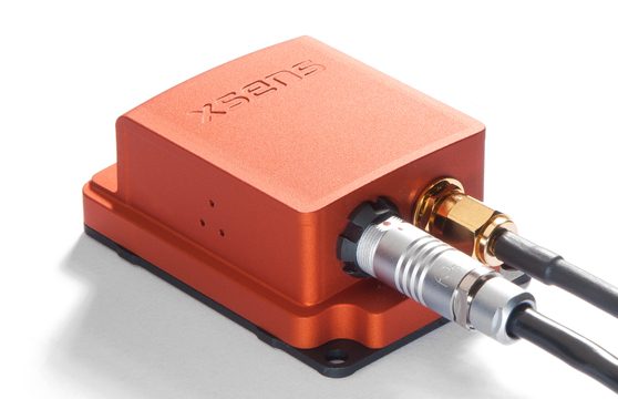 Representative IMU/INS
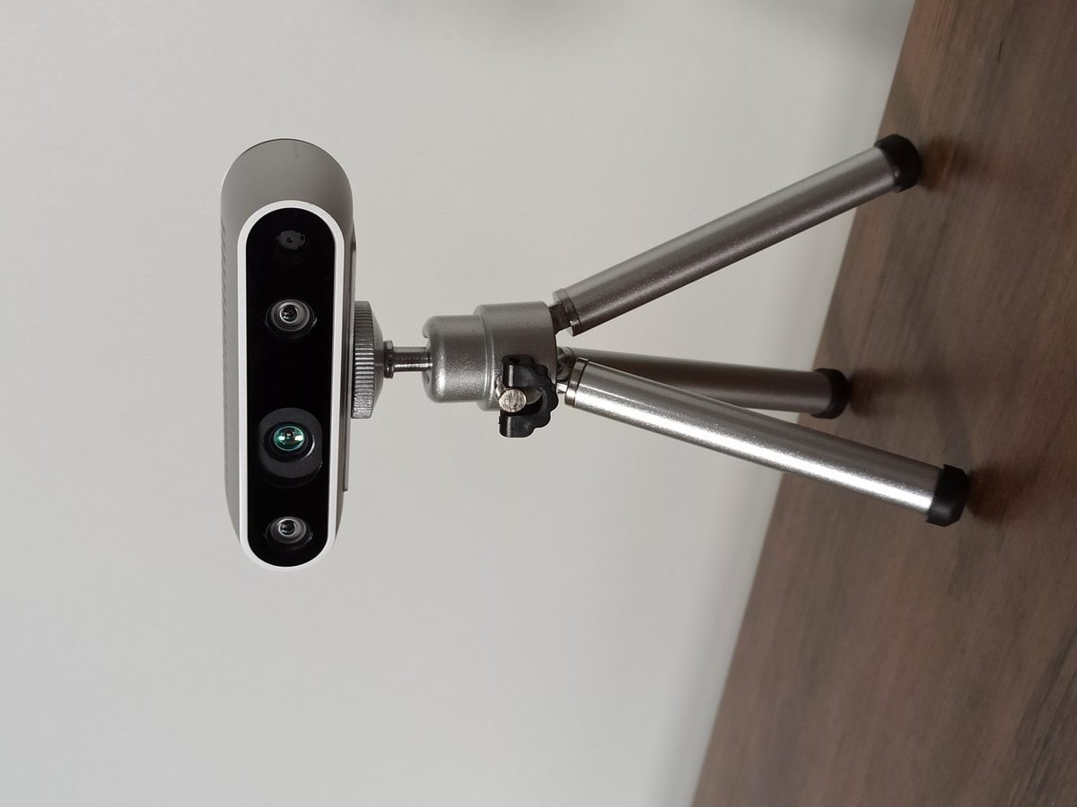 Representative depth camera
Images: Xsens MTi-G (Kallap85, CC BY-SA 4.0) and Intel RealSense D435 (Marc Auledas, CC BY-SA 4.0), Wikimedia Commons. They are representative sensors, not measured evidence or a recommended combined system.


Supplying PID, LQR, and MPC
PID may use raw filtered feedback, but its derivative term and an inner velocity loop often benefit from an estimate. LQR assumes multistate \hat{x}; under the separation-principle conditions, an LQR gain and Kalman estimator form an LQG architecture. Saturation, delay, and nonlinearity can still destroy real-world robustness. MPC also depends on a timely initial state and disturbance estimate; optimizing from a stale estimate or falsely small covariance creates a polished plan for the wrong world.
| Goal | Typical control | Estimator output needed | Failure response |
|---|---|---|---|
| Single speed/temperature loop | PID | filtered measurement / velocity estimate | stop integral on sensor loss |
| Local multistate stabilization | LQR/LQG | synchronized \hat{x} and validity | do not overtrust growing covariance |
| Constrained path/allocation | MPC | state, delay, disturbance, confidence | slow or stop on stale state/solver fault |
Robot timing and fault-safe operation
In ROS 2, distinguish measurement time from message arrival time. Updating the present with a late camera datum as if it were current pulls a robot toward its past. Choose and document a policy: rewind/repropagate history, reject delayed data, or separate low-level odometry from slower map corrections. ROS 2 transport and coordinate transforms described in ROS 2 Primer and Sensor Fusion Primer are preconditions outside the filter equations.
Monitor timeout, covariance ceilings, repeated innovation-gate failures, diverging bias, unavailable transforms, and deadline overruns. If all measurements vanish, do not run indefinitely on prediction alone. Select speed limiting, stop, redundancy, or operator handoff based on the application. Estimator reset can jump state, so controller references, integral states, and outputs need bumpless handling.
Implementation checklist
- Define state, measurement, input, frame, measurement time, and receipt time.
- Quantify observability plus required accuracy and maximum latency for each state.
- Record evidence for Q,R,P_0 from specifications, data, and tests.
- Monitor symmetry/definiteness of P, innovation, gates, and timeout.
- Inject dropout, outlier, relocalization, and bias-change cases.
- Define what PID/LQR/MPC receives when estimate quality degrades and verify independent safety action.
References
- Kalman, 1960: A New Approach to Linear Filtering and Prediction Problems
- MIT Underactuated Robotics: LQR
- ROS 2 Primer, Sensor Fusion Primer
What happens when a measurement is trusted more?
With the same prediction uncertainty, lower measurement covariance shifts the update toward the measurement. Unrealistic confidence can make estimates follow noise.
Comments
Please log in to post a comment
No comments yet.