Contents — find the section you need
A small executable model makes PID gain changes and actuator saturation easier to inspect. These results were calculated on September 7, 2026 with Python 3.12.3. They are numerical simulations, not measurements or an identified motor model.
Model and conditions
The plant is \ddot y+2\dot y+y=u. Output y and control u are normalized; time is in seconds. Initial output, velocity and integral are zero. The target is 1 from time zero, then 0.4 from 6 seconds. The step is 0.005 seconds over 0–12 seconds, giving 2,401 samples per case.
The controller is u=K_pe+K_iI-K_d\dot y_m, with e=r-y_m. Here y_m is the measured output. The derivative acts on it rather than the target. Baseline gains are K_p=3, K_i=2, K_d=1. Integration and differentiation explicitly use the time step; the plant uses semi-implicit Euler integration. See PID fundamentals for the principles.
Run the code
Save pid_lab.py in an empty working directory and run the following. It requires only the Python standard library and overwrites result files with the same names.
python3 --version
python3 pid_lab.py
It produces the CSV and summary JSON. To regenerate the figure, save and run plot_pid.py in the same directory; plotting was checked with matplotlib 3.6.3. CSV columns are scenario, time, target, output, control and integral.
Compare delay and saturation
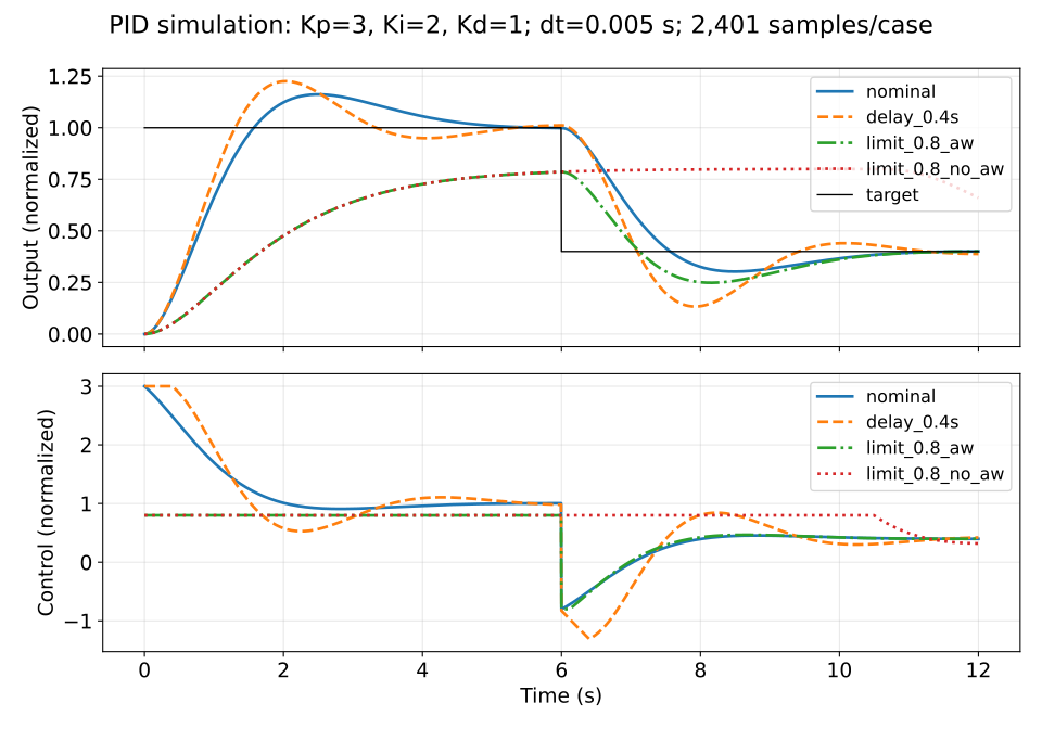
The upper plot shows output; the lower plot shows control. The black line is the target. Scenario labels match the CSV, and aw means anti-windup.
| Scenario | Change | Output at 12 s | Integrated absolute error |
|---|---|---|---|
| nominal | No delay, control limited to ±3 | 0.4008 | 1.7913 |
| delay_0.4s | Measurement delayed by 0.4 s | 0.3883 | 1.8860 |
| limit_0.8_aw | Control ±0.8, conditional integration | 0.4003 | 3.3424 |
| limit_0.8_no_aw | Control ±0.8, unrestricted integration | 0.6602 | 5.0996 |
Integrated absolute error uses left-rectangle integration over 0–12 seconds. Its units are normalized output times seconds, not physical position error in meters. Inspect oscillation and control effort as well as the final sample.
Anti-windup does not increase actuator capability
At equilibrium this plant has y=u, so a 0.8 control limit cannot reach a target of 1. If the error keeps accumulating, the integral can demand excessive input even after the target falls to 0.4. The code rejects integration that would drive further into saturation, while allowing integration that helps leave it.
This changes the controller's internal state, not the motor or supply capacity. Making the target achievable is a separate decision.
Change one gain at a time
from pid_lab import simulate
for kp in (1., 3., 6.):
    rows = simulate("gain", kp=kp)
    print(kp, max(row[3] for row in rows if row[1] < 6))
Compare the peak during the initial target interval. Then vary only ki, and then only kd, also recording maximum control effort. Larger gains are not universally better; repeat the comparisons with delay and saturation.
Limits and next checks
The model excludes measurement noise, friction, quantization, communication jitter and derivative filtering. Halve the time step: if the response changes substantially, investigate numerical approximation first. Do not copy these gains into hardware without identifying the plant and matching units and time scales. Continue to MPC to study constraints within the control problem.
Comments
Please log in to post a comment
No comments yet.