Contents — find the section you need
Change parameters and verify
Open the panel, then press Run to load Python. You can stop execution and reset parameters. Results are computed on this device. No Python installation is required.
Local execution steps below are optional for reproducing the source results; they are not required for the browser experiment.
Two browser experiments
The panel above is carbon and water accounting. Change light-period carbon uptake, all-day release and light-period duration to compare light, dark and daily carbon changes. The light period starts at hour zero. The lower sensitivity curve holds total conductance and total pressure fixed while varying leaf–air vapor-pressure difference; the point marks the selected condition. Its horizontal axis is not time. Defaults reproduce 9.2 gC and 0.1296 kg/(m² leaf·h).
Light timing, distribution and photon bands form a separate experiment. Open the panel below to reproduce equal-DLI schedules A/B, uniform U and uneven V, and spectra S1/S2.
The light panel covers a fixed 24-hour day and permits lighting across midnight. Upper bars show four cell PPFD values; bar width does not encode area. Uneven V multiplies nominal PPFD by 0.5, 1, 1 and 1.5. Choose area ratios 1:1:1:1 or 1:1:1:3; the mean is area-weighted. Lower bars split nominal PPFD into nonoverlapping 400–500, 500–600 and 600–700 nm photon bands. This is not a per-cell spectral measurement or optical simulation. Cell DLI, area ratios and the lighting time series are also in the data table.
Nominal DLI and band composition describe the nominal input; cell DLI and the area-weighted mean describe the spatial example. Changing areas leaves nominal DLI unchanged. At zero PPFD the positive-light duration is zero, and minimum/mean and band fractions are undefined (—).
Both experiments use synthetic accounting inputs, without predicting harvest, stomatal response, electrical energy or fixture performance. Carbon uptake is not inferred from PPFD through a coupled model. Bounds are teaching ranges, not crop recommendations. No Python installation is needed; local instructions below are optional. Save each entrypoint with its kernel to reproduce defaults locally: carbon/water entrypoint, kernel; light entrypoint, kernel.
Plants and their environment in CEA — connecting carbon, water, and control
Between an equipment setting and a plant response
A brighter lighting command does not establish an increase in carbon uptake. A lower humidity setting does not establish how much transpiration increased. Light and vapor pressure differences act through a plant whose condition and transport pathways also matter.
Following the CEA introduction, this guide treats a photosynthetic plant as a system that acquires carbon, transports water, and responds to its environment. Separate leaf exchange, whole-plant accounting, and room balances to understand the plant uptake and transpiration terms in the existing Labs.
In two illustrative calculations, daily carbon gain is 9.2 gC and halving total conductance at the same vapor pressure difference changes water transfer from 0.1296 to 0.0648 kg/(m² h). All inputs are synthetic. They are neither fitted crop parameters nor growing prescriptions.
Put photosynthesis and respiration into one carbon account
Photosynthesis uses light energy to incorporate carbon from CO₂ into organic matter. Respiration uses organic matter to provide energy for living processes and occurs in both light and darkness. Photosynthetic products can be allocated to roots and developing organs as well as leaves. Oregon State University's plant-growth guide explains these relationships.
For an illustrative group of plants, define carbon uptake as P_C and carbon release as R_C:
Both rates use gC/h, time uses hours, and the result uses gC: the mass of carbon, not CO₂ mass or fresh mass. This simplified account excludes harvesting, shed tissue, and carbon leaving through roots. Photorespiration is not modeled separately. When substituting measured data, redefine exactly which processes the uptake and release terms include.
In particular, do not insert a measured net assimilation rate as gross uptake and subtract the same leaf's respiration again. LI-COR's gas-exchange theory distinguishes net assimilation and respiration. Scaling an area-normalized leaf measurement to a plant group also requires an area convention, differences among leaves, and accounting for root and stem exchange outside that measurement.
Verify 16 light hours and eight dark hours
Prescribe whole-group uptake of 0.8 gC/h in light and zero in darkness, with release of 0.15 gC/h throughout the day. Sixteen hours is an accounting input, not a recommended photoperiod.
| Period | Uptake | Release | Carbon change |
|---|---|---|---|
| 16 light hours | 12.8 gC | 2.4 gC | +10.4 gC |
| 8 dark hours | 0 gC | 1.2 gC | −1.2 gC |
| 24-hour total | 12.8 gC | 3.6 gC | +9.2 gC |
Changing only the release rate to 0.25 gC/h gives 6.8 gC per day. The difference is independently checked as 24\times(0.25-0.15)=2.4 gC. No temperature-response function exists in this example, so the change cannot be attributed to a specified warming.
Nor is 9.2 gC a harvest-mass prediction. Conversion to dry matter needs a carbon fraction; fresh mass needs water content; marketable yield needs allocation, quality, and harvest criteria. The account provides only the carbon change over its defined period and boundary.
Stomata participate in both carbon and water exchange
CO₂ can enter the leaf for photosynthesis while water vapor leaves. Stomata affect both pathways, so responses that reduce water loss can also affect carbon entry. FAO describes transpiration through vaporization within the leaf and transport to the atmosphere, with stomatal opening and water supply among the relevant conditions. FAO: introduction to evapotranspiration
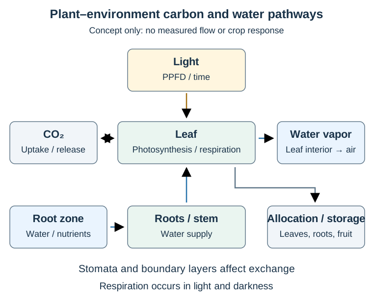
Conceptual diagram; arrow widths do not encode flow. Net CO₂ exchange can reverse with conditions, and photosynthesis and respiration can occur together in the light.
Leaf temperature matters to the vapor pressure difference. Approximating the leaf's internal air as saturated at leaf temperature T_l gives:
Here e_s is saturation vapor pressure and e_a is ambient vapor pressure. Air-based VPD calculated from air temperature T_a and RH is e_s(T_a)-e_a. It differs when leaf and air temperatures differ. The air-based indicator in the VPD/DLI Lab does not substitute for a leaf-temperature measurement.
Why VPD alone cannot determine transpiration
For an illustrative steady transfer from the leaf interior to ambient air, use:
g_{tw} is total water-vapor conductance, including stomatal and leaf boundary-layer effects, in mol/(m² s). Total pressure p and difference D_l must share units, here kPa. The resulting water-vapor flux E has units mol/(m² s). Area refers consistently to leaf area, not growing-floor area. Stomatal conductance alone cannot simply replace total conductance.
This is a dilute-vapor approximation using the mole-fraction difference D_l/p, not a complete instrument correction equation. The distinction between boundary-layer and stomatal resistance follows LI-COR's theory. FAO likewise separates plant-side and aerodynamic resistance and discusses effects of water status. FAO: resistance and evapotranspiration
With total pressure of 100 kPa and an approximate water molar mass of 0.018 kg/mol, compare these synthetic conditions:
| Condition | Total conductance | Interior-to-air difference | Water transfer |
|---|---|---|---|
| A: baseline | 0.20 mol/(m² s) | 1 kPa | 0.1296 kg/(m² h) |
| B: half the conductance | 0.10 mol/(m² s) | 1 kPa | 0.0648 kg/(m² h) |
| C: twice B's pressure difference | 0.10 mol/(m² s) | 2 kPa | 0.1296 kg/(m² h) |
A and B share a pressure difference but have different fluxes. A and C share a flux but describe different conditions. Neither VPD nor flux alone identifies stomatal state.
Conductance is prescribed here; the example does not predict stomatal responses to humidity. Actual resistance can change with plant water status, so drying the air does not establish a proportional increase in transpiration. Setting g_{tw}=0 gives zero flow only because it blocks every pathway in this model. It does not claim that real stomatal closure eliminates all water loss.
Connect root supply to the room balance
Water being present in the root zone does not establish an adequate supply rate into the plant. Root condition and water availability also need examination. Nutrient uptake likewise cannot always be reduced to water uptake multiplied by a fixed concentration. The subsequent root-zone guide will distinguish EC, pH, dissolved oxygen, and water temperature as separate measurements.
Observation boundaries matter. A falling tank level may combine plant uptake, evaporation, drainage, leakage, and refill operations. Water stored in the plant also allows uptake and transpiration to differ over a particular interval. Define the weighing or metering boundary with FAO's separation of evaporation and transpiration in mind. FAO: introduction to evapotranspiration
Transpiration in the moisture Lab, and uptake and respiration in the CO₂ Lab, were synthetic inputs. This guide does not replace them with a fitted plant-response model. That requires simultaneous environmental and plant-exchange measurements, area definitions, timestamp alignment, and validation under separate conditions.
Run the code and change one assumption
Save the calculation code and expected JSON. Python 3.10 or later and its standard library are sufficient.
The README records execution assumptions; the manifest records file sizes and SHA-256 hashes.
python3 experiment.py
python3 experiment.py --verify expected.json
python3 experiment.py --self-test
The first command prints JSON. The second compares every default numerical result with the expected file, failing on mismatches, omissions, or NaN. The third checks dark-period losses, time partitioning, unit conversion, zero flux, and invalid inputs.
The core calculation is short:
# Carbon: gC/h multiplied by hours, not a fresh-mass prediction.
delta_c = 0.8 * 16 - 0.15 * 24
# Water: mol/(m2 s) -> kg/(m2 h), pressure units cancel.
water = 0.20 * (1.0 / 100.0) * 0.018 * 3600
print(f"{delta_c:.1f} gC, {water:.4f} kg/(m2 h)")
Change the release rate passed by examples() near the bottom of the code, then change total vapor conductance in a separate run. The expected file remains a baseline, so a mismatch after changing inputs is expected. Subtracting respiration only during the light period overestimates this example by 1.2 gC. Mixing kPa and Pa in the water calculation introduces a factor-of-1000 error.
Records for the next environmental intervention
These are proposed experimental-design checks, not a crop-specific measurement standard.
| Comparison | Conditions to align or additional quantities to observe |
|---|---|
| Lighting change and carbon exchange | Leaf-level PPFD, CO₂, leaf temperature, time, leaf area, net/gross convention |
| Dehumidification and water exchange | Leaf and air temperatures, RH, airflow, water flows or mass, root-zone conditions |
| Environmental operation and growth | Cultivar, growth stage, treatment duration, dry/fresh mass definitions, controls and replicates |
| Disturbance and recovery | Records before, during, and after the event, sensor status, operation history |
A warmer leaf or slower growth alone does not identify a cause or diagnose disease. Compare duration and recovery, measurement error, and alternative explanations involving roots or airflow.
Next comes light quantity, timing, and distribution. Building on the VPD/DLI calculation, the next guide will distinguish conditions with the same DLI but different intensity and duration.
Light-environment design compares timing, shelf distribution, and wavelength mixtures that share the same DLI or PPFD.
Light in CEA — equal DLI, different timing, distribution, and spectrum
Equal DLI does not make two light environments identical
Providing 200 µmol/(m² s) for 16 hours or 400 for eight hours produces the same DLI: 11.52 mol/(m² day). Peak intensity and dark duration differ. A shelf averaging 200 also need not receive 200 everywhere.
Plant–environment foundations explained why a lighting setting does not uniquely determine carbon uptake or growth. This guide separates the light input into time, position, and wavelength. Every numerical example is synthetic, not a measured lighting map or crop prescription.
Keep PPFD, DLI, illuminance, and electrical power separate
| Quantity | Meaning on this page | What it does not establish |
|---|---|---|
| PPFD: µmol/(m² s) | Incident photon flux density at a measurement plane over 400–700 nm | Spectral composition or photons absorbed by leaves |
| DLI: mol/(m² day) | PPFD integrated over one day at that plane | Switching times or intermediate peaks |
| Illuminance: lx | Light weighted by human visual sensitivity | A source-independent conversion to PPFD |
| Power: W; energy: kWh | Electrical input and its time integral | Photons reaching the shelf or leaves |
Illuminance–PPFD conversion factors depend on the source.
DLI describes a daily integral. Purdue's DLI measurement guide recommends measurements at plant height and adjusting sensor height as plants grow.
The 400–700 nm measurement band does not define the entirety of plant responses. It does not imply that radiation outside the band has no biological effect. Instruments measuring ePAR over 400–750 nm also exist; state the band when comparing readings. Apogee's ePAR sensor description
Time: deliver the same integral with different schedules
For constant PPFD within each interval:
\Delta t_i uses seconds. The existing VPD/DLI Lab handles unequal intervals and missing-data checks. This example is limited to artificial-light schedules over a fixed 24-hour day.
| Synthetic condition | Lights on | PPFD while on | Light duration | Total dark time | DLI |
|---|---|---|---|---|---|
| A | 06:00–22:00 | 200 | 16 h | 8 h | 11.52 |
| B | 08:00–16:00 | 400 | 8 h | 16 h | 11.52 |
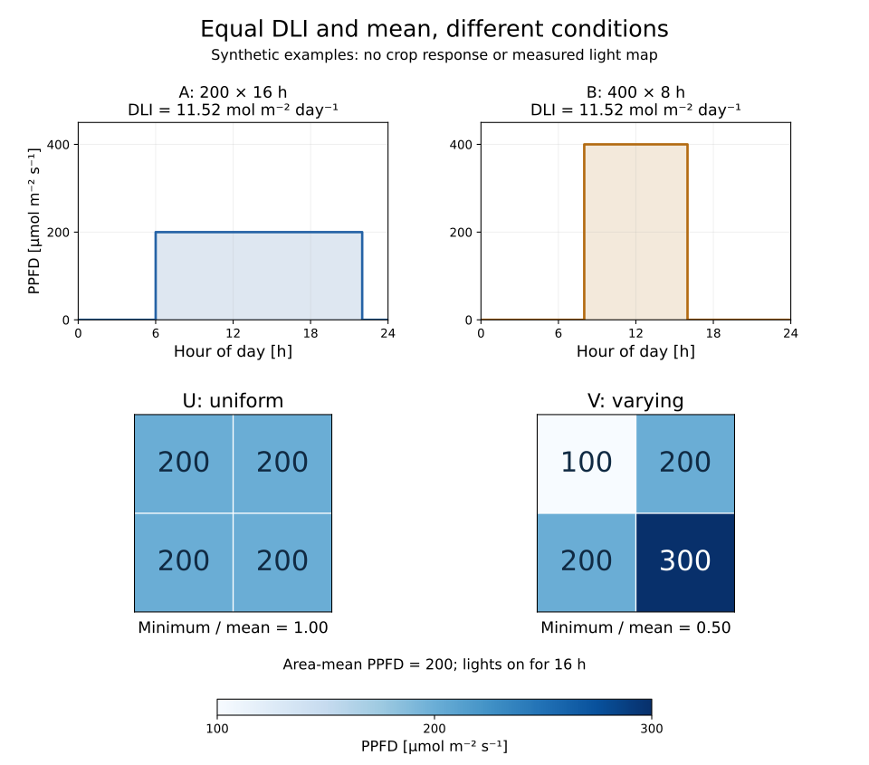
The upper areas represent equal integrals. The lower panels contain four equal-area synthetic cells, not measured lighting maps.
Equal integrals do not demonstrate equal photosynthesis or growth. In Elkins and van Iersel's original lettuce study (abstract), delivering the same DLI at lower PPFD over a longer photoperiod increased the daily integral of photosystem II electron transport. That reported metric does not establish yield or recommended day length for every crop. Our schedules A and B do not reproduce the study's experimental data.
Retain start and stop times, dimming history, peaks, and darkness alongside DLI. The same total light hours may describe continuous illumination or separated intervals. The code's light_hours reports total time with positive PPFD; it does not infer a biological photoperiod.
Space: find the dark areas hidden by an average
Assume four equal-area cells whose PPFD remains constant whenever the lights are on:
| Distribution | Cell PPFD values | Mean | Minimum/mean | Cell DLI after 16 hours |
|---|---|---|---|---|
| U: uniform | 200, 200, 200, 200 | 200 | 1.00 | 11.52, 11.52, 11.52, 11.52 |
| V: varying | 100, 200, 200, 300 | 200 | 0.50 | 5.76, 11.52, 11.52, 17.28 |
V has a mean DLI of 11.52, but its darkest cell receives half that amount. The average removes this distinction. Minimum divided by mean is a descriptive metric here, not an acceptance threshold.
If cells represent different areas a_j, calculate an area-weighted mean:
Two cells with area ratio 1:3 and PPFD values of 100 and 300 have a weighted mean of 250, rather than the arithmetic mean of 200. Treating point measurements as representative cell values requires an explicit grid, interpolation method, or represented-area assumption. Four measurements are not asserted to characterize a real shelf.
Repeat measurements at the same height, orientation, and coordinates. Preserve edge locations, points under fixtures, and structural shadows, and repeat after crop development. Incident PPFD on a horizontal empty shelf differs from light received and absorbed by tilted leaves. When moving a sensor around a greenhouse, retain a fixed reference to distinguish location effects from changing daylight.
Spectrum: different wavelength mixtures can share a PPFD
PPFD sums photons within a band and does not preserve their spectral distribution. These illustrative band-integrated photon flux densities both sum to 200, but the 400–500 nm fraction is 20% for S1 and 10% for S2.
| Synthetic spectrum | 400–500 nm | 500–600 nm | 600–700 nm | Total |
|---|---|---|---|---|
| S1 | 40 | 60 | 100 | 200 |
| S2 | 20 | 40 | 140 | 200 |
Each band uses µmol/(m² s); shared wavelength boundaries are counted once. These are not fixture specifications or performance rankings. State whether spectral fractions refer to photon counts or radiant energy and which wavelength range forms the denominator.
A photon's energy depends on wavelength, so photon fractions differ from fractions expressed in watts. A changing spectrum can also change a quantum sensor's measurement error. Apogee explains spectral error through differences between ideal and actual wavelength response and between calibration and measurement light sources.
For spectrum comparisons, preserve spectral measurements when available and record PPFD, photoperiod, leaf temperature, CO₂, and root-zone conditions. A color name or dimmer setting alone does not establish matching spectra.
Design measurement and energy records
The following records are proposed for comparing conditions:
| Record | Confusion it helps prevent |
|---|---|
| Sensor model, wavelength band, calibration date, source | Band and spectral-error differences |
| Plane, height, orientation, grid, area weights | Comparing different positions or surfaces as identical |
| Time, time zone, sampling interval, missing data | Incorrect integration or dark-time accounting |
| Dimming/switching history, shading, crop condition | Assuming the same command gives the same incident light |
| Meter boundary and integrated electrical power | Inferring electricity directly from PPFD |
A constant 100 W light running for 16 hours uses 1.6 kWh. A PPFD reading of 200 does not establish a 100 W input. Check dimming behavior, drivers, and the fraction of light reaching the shelf separately. If comparing cooling, dehumidification, and fan electricity too, align the equipment boundaries of the measurements.
Run the code and exercise failure cases
Download the code, expected results, README, and manifest. Python 3.10 or later and its standard library are sufficient.
python3 experiment.py
python3 experiment.py --verify expected.json
python3 experiment.py --self-test
The central arithmetic is:
a = 200 * 16 * 3600 / 1_000_000
b = 400 * 8 * 3600 / 1_000_000
darkest = 100 * 16 * 3600 / 1_000_000
print(f"A={a:.2f}, B={b:.2f}, darkest={darkest:.2f}")
In examples(), changing V's 100 to 50 changes both minimum and mean. To shorten B's lighting interval from 16:00 to 15:00, also move the next dark interval's start to 15:00. Changing only the light interval leaves a one-hour gap, which is rejected as missing coverage. Represent darkness explicitly with zero PPFD.
Tests cover equal DLI, interval subdivision, known cell doses, area weighting, darkness, the undefined ratio under zero illumination, invalid values, gaps/overlaps, and corrupted expected results. When every cell is zero, minimum/mean is 0/0; JSON reports null instead of inventing a ratio of zero or one. Numerical agreement does not validate crop response.
Next comes root-zone water and nutrients: separate EC, pH, dissolved oxygen, and water temperature, and connect each measurement to the operations that change it.
Controlled environment agriculture — connecting plants, light, air and water
Controlled environment agriculture (CEA) uses equipment and measurement to manage the environment around a crop. It includes greenhouses and indoor cultivation using artificial lighting. Instead of identifying CEA with a building called a plant factory, ask what the plant receives, what it returns to its surroundings, and which equipment changes those exchanges. The University of Arizona CEAC brings horticulture and engineering together in this field.
This guide concerns photosynthetic plants. Do not transfer its input/output model unchanged to fungi or fish production.
Greenhouses and indoor farms have different boundaries
| System | Light input | Connection to the outside | Separate in your records |
|---|---|---|---|
| Greenhouse | Sunlight, with optional supplemental light | Solar radiation, outside air and ventilation matter | Outside versus inside; sunlight versus supplemental light |
| Indoor farm with artificial lighting | Mainly installed lighting | Lighting schedules are controllable, but HVAC, water and people still cross the boundary | Lighting versus HVAC electricity; conditions at each shelf |
This comparison does not establish which system always uses less energy. Cornell's greenhouse and growth-chamber facilities distinguish greenhouses from chambers designed to isolate experiments from the surrounding environment. Check the actual control capabilities rather than inferring them from a facility name.
Put the plant at the center
Light, temperature, humidity, CO₂, water and nutrients must be considered together. The environmental factors described by Missouri Extension can be organized into a measurement-and-equipment map:
| Part | Plant-side question | Example observations | Example equipment |
|---|---|---|---|
| Light | What reaches the leaves? | PPFD, lighting duration | Lights, shading |
| Air | What surrounds the leaves? | Air temperature, relative humidity, CO₂ | HVAC, ventilation, dehumidification |
| Root zone | What water, nutrients and oxygen reach the roots? | Water flows, water temperature, EC, pH | Pumps, irrigation, drainage |
| Crop | How did growth respond? | Fresh and dry mass, leaf count, quality | Outcomes to evaluate, not directly commanded values |
Keep measurements, setpoints and crop outcomes separate. A 25°C air-conditioning setting does not prove that the air around the leaves was 25°C. One humidity measurement cannot establish uniform conditions across every shelf. Electrical conductivity (EC) relates to ions in solution; it is not a measurement of each nutrient concentration. This map does not replace crop-specific management or calibration procedures.
A small boundary exercise
Consider a fictional room containing a lit growing shelf, a water tank and HVAC. The following is an explanatory example, not facility data. Draw the boundary around the whole room.
| Exchange | Inputs | Outputs or accumulation | Recording distinction |
|---|---|---|---|
| Energy | Electricity for lights, HVAC and pumps | Heat leaving or accumulating inside | Power in kW versus energy over an interval in kWh |
| Water | Makeup water | Drainage, recovered condensate, water retained in plants and the room | Internal reuse versus external supply |
| Material | Seedlings, fertilizer, incoming air | Harvest, waste, outgoing air | Whole-room totals versus tank-only totals |
Pumping water from the tank to roots inside the room is not itself an external water input. Draw the boundary around the tank instead, and the same flow becomes an output. Explaining this distinction helps prevent confusion between water circulation and water use.
For an arithmetic check, a constant 0.2 kW lighting load over 16 hours consumes 3.2 kWh. This assumed value covers only lighting, not total facility electricity or the light reaching a leaf.
Separate light intensity from daily light quantity
PPFD expresses photosynthetically active photon flux per unit area, commonly in μmol m⁻² s⁻¹. DLI integrates that quantity over a day, in mol m⁻² day⁻¹. Purdue's DLI guide explains the distinction between instantaneous and daily quantities.
Assume a constant PPFD of 200 μmol m⁻² s⁻¹ for 16 hours and zero light otherwise. DLI is 200 × 16 × 3600 ÷ 1,000,000 = 11.52 mol m⁻² day⁻¹. This is a different quantity from the previous 3.2 kWh example. Electrical power alone does not determine PPFD.
For real time series, preserve timestamps and intervals. Missing samples are not proof that the lights were off. Equal daily totals also do not establish identical light delivery throughout the day.
Move from measurement toward control
Start with temperature measurement: record location, units and timestamps. Then use sampling principles to ask whether the recording interval captures relevant changes. Keep changed settings, surrounding conditions and crop responses in separate records.
The next learning targets are air vapor pressure deficit (VPD), derived from air temperature and relative humidity, and DLI integration from light time series. The VPD/DLI Lab now provides synthetic CSV and executable Python. A browser panel is also available. This guide's arithmetic examples are not a working crop simulator.
To check your understanding, list what a record saying “lights on for 16 hours” leaves unknown. Without light intensity, measurement location and incoming daylight, DLI is undetermined. Likewise, a temperature setpoint does not establish the plant's experienced environment. These distinctions turn an equipment list into a system you can investigate.
Continue with the plant side
Plant–environment foundations connects photosynthesis, respiration, and transpiration to carbon and water accounts, showing what equipment settings alone cannot determine.
Comments
Please log in to post a comment
No comments yet.