Contents — find the section you need
Change parameters and verify
Open the panel, then press Run to load Python. You can stop execution and reset parameters. Results are computed on this device. No Python installation is required.
Local execution steps below are optional for reproducing the source results; they are not required for the browser experiment.
Two browser experiments
The panel above runs cooling response: change the actuator time constant, lighting sensible heat and cooling capacity. The 0/300/900/1800-second presets keep the other inputs at their published baseline. Temperature and command/delivered cooling are plotted separately. No Python installation is required; the local reproduction commands below are optional.
The coupled-control panel runs both ON/OFF and PI for every parameter change. Six separate bar plots compare band violations, cooling/dehumidifier-command overlap, cooling heat, water removal and actuator variation. Each plot has its own units and scale. A/B saves an entire pair of controller results, so the controller comparison and the change of conditions remain distinct. Full metrics, numeric series, downloads and shared conditions are available in both Labs.
Cooling response retains the original 12-hour model, 10-second room Euler step and exact interval-mean first-order actuator update. Lights switch at 2 and 8 hours; initial/setpoint temperature is 24°C, outside 22°C, base heat 800 W, heat capacity 12 MJ/K, UA 300 W/K and fixed PI gains 0.6 and 0.0004. All original samples are plotted, including the final held command. The evaluation band remains 23–25°C. Error and band time use interval starts; extrema include endpoints. The model excludes moisture and sensor lag.
Coupled control retains 24 hours with 60-second explicit steps, lights at 08–24, initial 24°C/RH70%, 300 m³, 12 MJ/K, UA 450 W/K and 0.05 m³/s ventilation. Outside temperature is 21±6°C and RH60%; lit/dark transpiration is prescribed at 2/0.35 kg/h. ON/OFF thresholds remain 23.5/24.5°C and RH65/75%; PI targets remain 24°C/RH70% with the original fixed gains and conditional integration. Violations use updated states against 23–25°C and RH60–80%. Total variation sums absolute command changes, not switching counts. The original overlap metric counts positive cooling and dehumidifier commands even if indoor reheat is set to zero.
The coupled model caps water against saturation at the previous temperature before updating temperature; it does not re-equilibrate condensation after cooling or return condensation heat. Cooling is sensible-only; drying is a prescribed mass sink with separate reheat. It has no coil model, actuator delay, sensor dynamics or CO₂ coupling. The two Labs are distinct synthetic experiments, not interchangeable configurations. Thermal kWh is not electricity, and bounds/presets are teaching assumptions rather than crop settings or equipment sizing. Original kernels, configurations, ZIPs and reference results are preserved.
cooling: experiment.py · cooling_kernel.py · config.json
coupled: experiment.py · coupled_kernel.py · config.json
CEA Temperature and Humidity Control — why cooling, drying and ventilation interact
Temperature and RH can have separate targets, but actuators rarely affect only one quantity. A cooling coil removes sensible heat and may condense water below the dew point. Some dehumidifiers collect water while returning sensible heat indoors. Ventilation carries temperature, vapour and CO₂ together according to outdoor conditions. Independent temperature and humidity switches can therefore fight each other.

Diagram: Duskcoil. A responsibility-level schematic independent of a specific equipment arrangement.
Separate states from commands
The thermal-balance Lab stores room temperature T; the moisture-balance Lab stores vapour mass m_v. RH remains derived rather than becoming another conserved state.
| Command | Typical temperature effect | Typical moisture effect | Measure together |
|---|---|---|---|
| Cooling | Removes sensible heat | Condenses below coil dew point | Supply temperature, condensate |
| Dehumidification | May reheat indoors | Removes water | Collected water, heat rejection, power |
| Ventilation | Heats or cools by outdoor difference | Adds or removes vapour | Outdoor T/RH, CO₂, airflow |
| Heating/reheat | Adds sensible heat | No direct mass change | RH falls through temperature change |
| Humidification | Evaporation may consume latent heat | Adds water | Feed water, droplets, hygiene |
U.S. DOE HVAC guidance distinguishes sensible and latent control and describes overcooling/reheat interactions. Oklahoma State University Extension likewise treats greenhouse ventilation as part of both temperature and humidity management.
Supervision prevents accidental conflict
Humidity-driven cooling followed by low-temperature heating can run cooling and heating together. That is not automatically wrong—deliberate reheat can reduce humidity—but intent, allowed duration and energy cost must distinguish a designed mode from controllers cancelling each other.
A minimal supervisor makes priorities explicit:
- Sensor faults, condensation and equipment-protection constraints
- Hard temperature and absolute-moisture limits
- Normal target bands and hysteresis
- Conditions allowing or forbidding simultaneous operation
- Power limits and side effects such as ventilation CO₂ loss
Acceptance conditions for controller comparison
On/off, rule-based and PI comparisons must share weather, prescribed transpiration, LED schedule and initial state. Fix actuator capacity, minimum run/off time, delay, saturation, and power or collected-water accounting. Report time outside temperature and RH bands, condensation, switching count, simultaneous heating/cooling time and energy separately. One average error is insufficient.
Reject runs that clip sensors silently, hold missing values without declaring it, or give only one controller future weather. Also reject runs that violate the underlying energy or water residual checks.
This is a control-design entry point, not crop-specific settings or equipment recommendations. The next implementation should couple only thermal and moisture states in one simulation while keeping CO₂ as a separate monitored constraint.
References
- Grid-interactive Efficient Buildings: HVAC (U.S. DOE)
- The Hobby Greenhouse (Oklahoma State University Extension)
- Assessing the Risk of Disease in Greenhouses (Penn State Extension)
Temperature and Humidity Sensors — Placement, Response, and Calibration
Which temperature does the controller see?
The cooling response Lab separated cooling command from delivered cooling. Its controller still received the current model temperature directly. Moving toward a facility requires separating the physical environment, the sensor reading, and the value passed to control as well.
Consider an ideal air-temperature step from 24°C to 26°C and a measurement system modeled by a 60-second first-order time constant. After 30 seconds, its reading is 24.787°C. Comparing that reading with 25°C misses an exceedance already present in the input. This is an illustrative analytical calculation, not facility data or a product specification.
This article is a measurement-design guide. It does not rerun the previous closed-loop Lab or rank products, and its example threshold is not a crop recommendation.
Give each measurement location a purpose
A single average of growing-zone, supply-air, and return-air readings removes information about where a change occurred. Define the quantity and location of interest before choosing an aggregation rule. The following investigation plan is an editorial proposal, not a universal sensor-count requirement.
| Purpose | Example locations to compare | Interpretation |
|---|---|---|
| Describe the growing zone | Different shelf heights, rows, and distances from supply air | Preserve individual histories and differences |
| Diagnose HVAC action | Supply and return air | Keep these distinct from growing-zone readings |
| Find local departures | Door, wall, and rear of a shelf | Do not hide an extreme location in an average |
| Investigate instrument differences | Temporary co-location | Reduce location differences before comparing instruments |
Sensirion's design guide identifies representative placement, enclosure air exchange, and thermal influences as system-level concerns. A sensor's standalone accuracy does not establish installed accuracy.
For a survey, record lighting, fan operation, and crop growth stage, then compare positions under corresponding operating conditions. If a portable sensor moves between positions, retain a fixed reference point: a room-wide change during the survey can otherwise look like a spatial difference. Exchanging two instruments between positions can help, but conditions may change during the exchange. Combine swaps with co-location to narrow the cause.
Separate response time from logging interval
Reading a value every second does not establish a one-second physical response. Temperature and RH can also respond differently. Check the definition and installed configuration; the design guide discusses response in terms of reaching approximately 63% of a step.
For this example only, let target temperature be T, measured temperature be T_m, and measurement time constant be \tau_s:
With initial equilibrium at 24°C, a constant input of 26°C, and \tau_s=60 seconds, the solution is T_m(t)=26-2\exp(-t/60).
| Time after step | Target temperature | Reading | Target minus reading |
|---|---|---|---|
| 30 s | 26.000°C | 24.787°C | 1.213°C |
| 60 s | 26.000°C | 25.264°C | 0.736°C |
| 180 s | 26.000°C | 25.900°C | 0.100°C |
The reading reaches the illustrative 25°C threshold after about 41.6 seconds. Discrete logging can postpone detection until the next sample. This model begins responding immediately; it is different from pure dead time, during which no response occurs.
Save the following standard-library Python code as sensor_example.py and run python3 sensor_example.py to reproduce the table and threshold-crossing time. It reads and writes no external files.
from math import exp, log

initial, final, tau = 24.0, 26.0, 60.0
for seconds in (30, 60, 180):
    measured = final + (initial - final) * exp(-seconds / tau)
    print(f"{seconds:3d} s: {measured:.3f} C, gap {final-measured:.3f} C")
threshold = 25.0
crossing = -tau * log((final - threshold) / (final - initial))
print(f"threshold crossing: {crossing:.1f} s")
A real room need not change as a step, and an installed measurement system need not have a single time constant. When investigating response from logs, account for reference-instrument dynamics and timestamp alignment. The interval between a cooling command and a changed reading combines actuator, air-transport, and measurement effects; that interval alone cannot identify each contribution.
Preserve the value before and after filtering
If control applies a moving average or another filter, log both the acquired instrument output and the processed control input. The acquired output may already include internal processing. Preserve the filter settings as well.
To extend the previous Lab, use T_m-T_{sp} as the PI error while retaining the model's true temperature T for evaluation. Count time outside the band separately for measured and true temperature. The calculation here has no feedback loop, so it makes no numerical claim about resulting oscillation or additional overshoot.
In a facility, true temperature is not directly available. Independent reference measurements also carry uncertainty; document the reference instrument, position, and calibration information when reporting a comparison.
Treat temperature and RH as a pair
Relative humidity expresses vapor pressure relative to saturation vapor pressure at the relevant temperature. For VPD calculations, use temperature and RH representing the same air and align their timestamps. Combining shelf temperature with supply-air RH does not measure shelf VPD.
A heated humidity probe requires distinguishing the heated sensing region from ambient air. Vaisala's warmed-probe note describes using an additional ambient-temperature measurement to obtain ambient RH. Follow the selected instrument's output specification instead of treating every heated-probe output as growing-zone temperature and RH.
When supplying values to the VPD Lab, distinguish an air-temperature calculation from a leaf-to-air calculation using leaf temperature. Without a leaf-temperature measurement, do not label the air-based result as a measured leaf condition.
Keep calibration, adjustment, and placement surveys separate
Vaisala's calibration note distinguishes comparison against a reference from adjustment of an instrument. Agreement at one point does not verify the entire operating range. Choose comparison points and acceptance limits with the operating range and reference uncertainty in mind.
Record instrument ID, the reading before adjustment, the reference reading, stabilization conditions, and the date. If adjustment occurs, add the setting changes and subsequent comparison. Discarding the original discrepancy makes earlier growing logs harder to assess.
Two instruments agreeing does not exclude a shared bias. Calibration also does not establish that the installed position represents the growing zone. Complete the instrument comparison and location survey as separate tasks.
Define the record passed to control
The following fields are a proposed logging design, not a measured dataset.
| Field | Purpose |
|---|---|
| Measurement and reception timestamps, time zone | Separate communication delay from environmental change |
| Instrument ID, location ID, installed height | Track replacements and moves |
| Temperature, RH, units, instrument status | Identify heating modes and invalid readings |
| Filter settings and processed control value | Reconstruct the controller's input |
| Lighting, fans, cooling command and operating state | Align disturbances with equipment response |
| Calibration, replacement, and cleaning history | Explain discontinuities around maintenance |
Holding the last reading during a communication failure can produce a reassuringly flat display. Pass sample age and validity alongside the value. Define the stale-data limit and the resulting control action for the actual equipment and crop, then verify that behavior during commissioning.
Before the next experiment, investigate instrument differences through co-location, spatial differences through a location survey, and latency from acquisition to control input. Together, those records support deciding whether to change the controller or improve the measurement process.
Cooling-Response Lab — separate the PI command from delivered cooling
Equal cooling capacity does not mean equal response
The previous coupled-control comparison assumed that a change in command immediately changed cooling and drying capacity. This experiment isolates sensible cooling and lets delivered capacity follow the command gradually. It is a synthetic room model, not a measured cultivation facility.
Over the same 12 hours, increasing the actuator time constant from zero to 900 seconds changes integrated absolute temperature error from 2.287 to 4.351 K·h and minimum temperature from 23.419 to 23.044°C. Both cases stay within the chosen 23–25°C band. A binary pass/fail band check alone therefore hides a substantial difference in response.
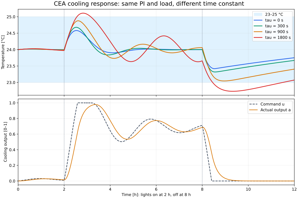
Figure: Duskcoil, generated from the distributed Python simulation. The red 1800-second trace is a stress case. The band is an experimental assumption, not a crop recommendation.
A deliberately smaller experiment
This is a separate experiment to isolate actuator response, rather than a one-parameter rerun of the previous coupled model. It excludes humidity, transpiration, dehumidifier reheat and CO₂. All cases use 22°C outside air, 800 W background heat, and an additional 8,000 W of lighting-related sensible heat between hours 2 and 8. The 8,000 W is not an estimate of lighting electrical demand.
| Setting | Value | Interpretation |
|---|---|---|
| Effective thermal capacitance | 12 MJ/K | Synthetic room and contents, not air alone |
| Envelope conductance | 300 W/K | Heat transfer proportional to indoor/outdoor difference |
| Maximum cooling | 12 kW | Sensible heat removal, not electricity |
| Initial temperature and setpoint | 24°C | Identical in every case |
| Evaluation band | 23–25°C | Acceptance criterion for this experiment |
| Simulation and control interval | 10 seconds | Light transitions align with the grid |
| PI gains | 0.6 K⁻¹; 0.0004 K⁻¹s⁻¹ | Fixed synthetic settings |
| Actuator time constant | 0, 300, 900 seconds | The variable under comparison |
DOE's sensible/latent separation project describes technology that handles temperature and moisture loads separately. This room model does not reproduce that equipment; moisture control and electricity require additional models and evaluation.
Give command and delivered output separate variables
Define error so that a temperature above setpoint increases cooling. The PI output clipped to 0–1 is command u. Delivered cooling as a fraction of maximum capacity is a.
This is a first-order lag. Under a constant command, one time constant covers about 63.2% of the requested change. A 900-second time constant does not mean that nothing happens for 900 seconds: that would be dead time. Delivered output starts at zero; only the zero-time-constant case follows the command instantaneously.
The room uses a sensible-heat balance:
The code holds the command for each ten-second interval and calculates the actuator's endpoint and interval mean analytically. The room temperature uses forward Euler with interval-mean cooling. This avoids counting the endpoint cooling rate as though it had been delivered throughout the interval.
The PI controller uses conditional integration: it freezes the integral when the unconstrained command is above its upper limit and the error would drive it further into saturation, but allows integration that releases saturation. MathWorks distinguishes this method from tracking the actual actuator output. Only conditional integration is implemented here; it does not itself compensate actuator dynamics.
Compare metrics over the same interval
| Time constant | Minimum °C | Maximum °C | Outside band h | Absolute error K·h | Cooling heat kWh |
|---|---|---|---|---|---|
| 0 seconds | 23.419 | 24.580 | 0.000 | 2.287 | 51.572 |
| 300 seconds | 23.319 | 24.679 | 0.000 | 2.751 | 51.953 |
| 900 seconds | 23.044 | 24.877 | 0.000 | 4.351 | 53.072 |
| 1800 seconds, stress case | 22.730 | 25.110 | 3.650 | 6.880 | 54.380 |
Integrated absolute error accumulates |T-T_{sp}|, so warm and cold deviations cannot cancel. Band duration and error use the temperature at the start of each interval: they are ten-second approximations. Minima and maxima include all grid endpoints, including the initial and final state.
At lights-off, sensible heat input drops immediately while delivered cooling decays gradually. Match the lower panel's remaining output after the command decreases with the upper panel's cold excursion. Increased cooling heat cannot be directly interpreted as increased electricity or cost: there is no cooling COP, pump or fan model.
Run, then change one condition
Extract the reproducible ZIP into an empty directory. Calculation and tests require only Python's standard library; validation used Python 3.12.
python3 reproduce.py
python3 -m unittest -v
python3 experiment.py config.json --tau 900 --csv trace-local.csv
python3 experiment.py config.json --tau 1800
reproduce.py verifies distributed file hashes and recalculates the saved 0-, 300- and 900-second cases. CSV export refuses to overwrite an existing file. The final CSV row carries the preceding held command; it does not represent a new control update at the endpoint.
Individual downloads: configuration, calculation source, reference results, 1800-second result, 900-second CSV, and manifest.
First try 1800 seconds without changing gains. It spends 3.650 hours outside the band. This means failure of the chosen acceptance criterion, not divergence or a demonstrated equipment fault. Then return to 900 seconds and change dt_s to 5 to inspect discretization effects. Changing every condition together obscures the cause of improvement.
Numerical correctness and facility suitability are different checks
Ten tests cover the analytical first-order response, interval subdivision, actuator bounds, integral freeze/release, constant-heat known solution, heat-balance residual, reference outputs, invalid input, half-step convergence and the stress-case band violation. Across the three standard cases, halving the step from ten to five seconds changes extrema, absolute error and cooling heat by less than 0.03°C, 0.03 K·h and 0.03 kWh respectively. Numerical convergence does not establish that the synthetic parameters represent a facility.
For a real installation, collect command histories and measurements that can estimate delivered cooling, then separate identification and validation data. Sensor lag, minimum run times, staged operation, dead time and humidity coupling are further extensions. Crop setpoints, disease risk and energy-saving percentages are not outputs of this experiment.
Continue reading
Temperature and humidity sensors examines placement, measurement response, and calibration before passing readings to control.
Coupled-Control Lab — compare on/off and PI under identical disturbances
Start with the result
Under the same synthetic 24 hours, PI reduces total actuator variation from 34.0 to 2.853 and cooling removal from 182.233 to 178.854 kWh. But temperature violation increases from 7.95 to 10.02 h, and simultaneous cooling plus dehumidifier reheat increases from 9.37 to 14.65 h. This run does not establish PI as superior.
Diagram: Duskcoil. Shared system boundary for the controller comparison.
Shared conditions
The thermal and moisture balances are combined with only two states: room temperature T and vapour mass m_v. Weather, LEDs, prescribed transpiration, initial state, 60-second step, 14 kW cooling and 2.5 kg/h drying are identical. The synthetic dehumidifier returns 1.8 kW sensible heat indoors. CO₂ remains separate.
Hysteresis switches around 24±0.5°C and 65/75% RH. PI outputs saturate at 0–1 and use conditional anti-windup. Gains are synthetic, not tuned equipment settings.
| Metric | On/off | PI |
|---|---|---|
| Outside 23–25°C | 7.95 h | 10.02 h |
| Outside 60–80% RH | 4.25 h | 4.25 h |
| Cooling removal | 182.23 kWh | 178.85 kWh |
| Dehumidified water | 24.25 kg | 23.06 kg |
| Simultaneous cooling/reheat | 9.37 h | 14.65 h |
| Total actuator variation | 34.0 | 2.85 |
As DOE guidance explains, sensible and latent control can involve overcooling and reheat. Lower energy alone does not settle the design when violations or simultaneous operation rise.
Run and verify
Extract the ZIP:
python3 experiment.py config.json > result.json
python3 -m unittest -v
See config.json, expected.json, and experiment.py. Eight tests cover both controllers, determinism, energy/water residuals and invalid inputs.
Before tuning gains, fix acceptance bands, metric weights, simultaneous-operation limits, electric conversion and actuator delays. Real deployment must separate identification and validation data. This article does not provide crop settings, real equipment savings or a guarantee of PI superiority.
The cooling-response follow-up separates command from delivered cooling and varies only the actuator time constant.
Comments
Please log in to post a comment
No comments yet.