Contents — find the section you need
Change parameters and verify
Open the panel, then press Run to load Python. You can stop execution and reset parameters. Results are computed on this device. No Python installation is required.
Local execution steps below are optional for reproducing the source results; they are not required for the browser experiment.
Try the projected-area experiment in your browser
The panel above runs the synthetic image experiment without installing Python. Choose the clean, green-tag, dim or clipped scene; change minimum brightness V, region of interest and mm/pixel. Nine presets include all seven published conditions, an undersized ROI and an empty selection. Presets reset every input; changing the threshold manually also changes the recovered-dim case.
Inspect the input, in-frame reference, extracted mask and error overlay. Red marks false positives and blue marks false negatives. A brown boundary marks a selected ROI on the input. Save a result as A and change one input to compare images and metrics at the same display scale. The data table gives horizontal pixel runs (zero-based x/y and length); they reconstruct each image region exactly, without downsampling. Share conditions or download result JSON to retain the experiment.
Images remain the original 320×240 geometric scenes, with no real-photo upload or camera input. The original NumPy geometry and measurement functions are reused unchanged. The browser replaces only OpenCV conversion/range selection with a verified lookup of its three fixed RGB colors: background (235,235,235), target (50,160,65) and dim target (20,60,25). Their OpenCV 4.6.0 uint8 HSV values are (0,0,235), (64,175,160) and (64,170,60). This is not a general-purpose HSV converter. H 35–85 and S 80–255 stay fixed; V minimum is adjustable from 0 to 255, inclusive. No morphology is applied.
The fixed tag-excluding ROI is (50,20,230,190); the small ROI is (140,60,20,30), in x/y/width/height pixels. Neither adapts to a plant. Scale ranges from 0.1 to 1.0 mm/pixel as an assumed reference-plane conversion, not a calibration. The image stays the same when scale changes. touches_frame appears as 1 for yes and 0 for no; an empty selection has undefined precision (—). Perfect IoU for a clipped scene still says nothing about portions outside the image. These outputs do not measure biomass, growth, stress or real leaf-surface area.
Original downloads and saved baselines remain unchanged. Local reproduction instructions below are optional. The browser adapter uses NumPy without OpenCV; save its entrypoint, kernel and palette together to run it locally with NumPy installed.
CEA sensing and flow — where to measure CO₂ and nutrient solution
Equal displays can refer to different places and times
Reservoir DO differs from DO at a growing channel's outlet. Before attributing the difference to root oxygen consumption, check whether the sensors observe comparable times, whether calibration is consistent, and whether the sample changes in transit.
The root-zone guide separated EC, pH, DO and water balance. This article asks where and how to compare them. It reuses the lag and calibration concepts from the temperature/humidity sensor guide, adding issues specific to CO₂, nutrient solution and flow.
The placement table and investigation procedure below are our proposed design approach. They are not facility measurements, required sensor counts or universal crop alarm thresholds.
Decide which differences you need to observe
| Target | Example comparison points | Companion records |
|---|---|---|
| Crop-zone CO₂ | Near canopy, supply air, exhaust or return air | Height, dosing, ventilation, doors, temperature and RH |
| EC, pH and water temperature | Mixed reservoir, growing-channel inlet and outlet | Source water, additions, volume and circulation |
| DO | Reservoir, near roots, channel outlet | Temperature, aeration and sensor technology |
| Liquid flow | Makeup, selected branches, discharge | Flow, location and valve state |
| Level and pressure | Reservoir, upstream/downstream of a filter | Level-to-volume relationship, pressure reference and elevation |
| Air movement | Front/back of shelves and different heights | Probe orientation, averaging duration and fan state |
Use permanent points for monitoring and portable measurements for mapping. Retain a fixed reference to distinguish time variation during a moving survey. Assign location IDs independently of sensor IDs so replacements do not break location history.
Does CO₂ self-calibration fit the growing conditions?
A measurement immediately beside a CO₂ outlet should not automatically represent the entire canopy. Record relationships to injection, supply/exhaust air and human breath. A point diagnosing the dosing equipment serves a different purpose from one assessing crop conditions.
Check the calibration algorithm. The 2018 Sensirion SCD30 field-calibration note describes ASC using a minimum concentration corresponding to 400 ppm and requiring regular exposure to that concentration.
Our inference is that continuously enriched rooms may not satisfy this assumption. This concerns the documented algorithm, not every CO₂ sensor. Follow the selected model and firmware's instructions and plan comparison with reference gas or a calibrated instrument. The historical 400 ppm assumption is not a guaranteed present-day outdoor calibration value.
Temperature/RH outputs built into a CO₂ device may describe its enclosure rather than representative canopy air. Distinguish environmental compensation inputs from measurements used to evaluate the crop environment.
EC, pH and DO need different checks
The USGS multiparameter-instrument manual connects storage, maintenance, calibration, measurement and reporting. Its natural-water scope does not establish crop setpoints or suitability for a particular nutrient solution.
The following proposed checklist applies that general approach; actual procedures and solutions must match the instrument documentation.
| Parameter | Items to verify |
|---|---|
| EC | Conductivity standard and temperature, expected range, cell constant and temperature compensation |
| pH | Buffers appropriate to the range, temperature, electrode/junction condition and storage |
| DO | Optical or electrochemical method, calibration conditions, pressure/salinity compensation, membrane or cap condition |
| All | Before-adjustment error, results after cleaning/adjustment, standard identity, date and stabilization time |
Agreement in a standard does not establish representative readings after installation. Investigate bubbles, deposits, stagnant liquid and local concentration differences immediately after additions.
DO technology matters. YSI's measurement guidance explains that optical sensors do not consume oxygen and have no measurement-principle stirring requirement, although flow can improve response time. Do not assume identical flow requirements for electrochemical and optical devices. Even an optical sensor still needs to sample liquid representative of the intended root environment.
A sampling line brings older liquid to the sensor
A remote flow cell separates display time from conditions at the sampling point. For a synthetic line volume of 0.50 L and constant flow of 0.25 L/min, assume ideal displacement with no mixing or dispersion:
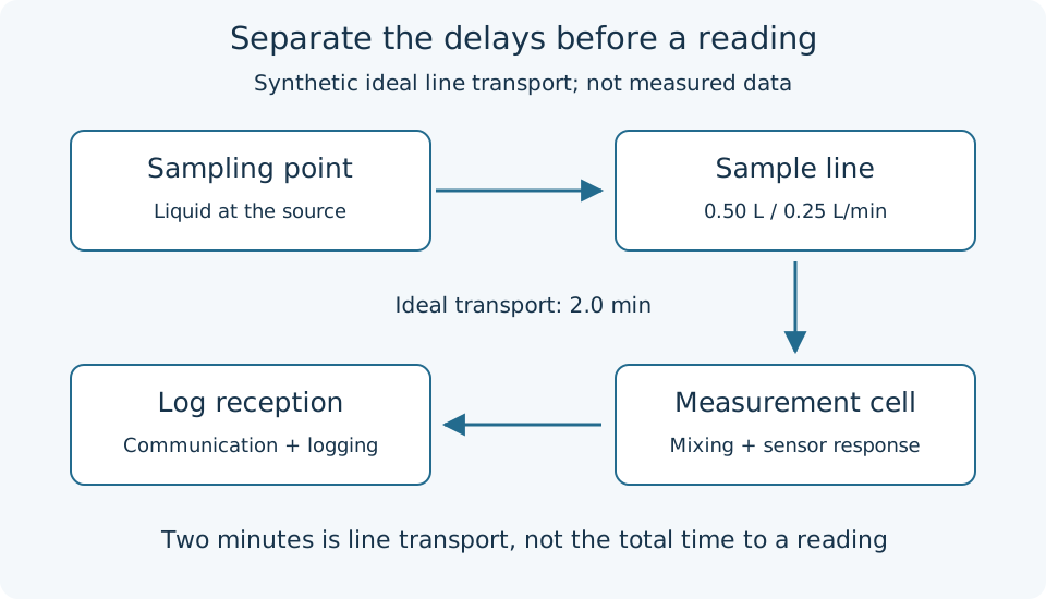
The two minutes describe ideal line transport only. Cell mixing, sensor response and communication delay are additional effects.
Doubling flow to 0.50 L/min reduces this ideal time to one minute. Real lines and cells mix; temperature and gas exchange can also change the sample. Shifting timestamps by two minutes does not necessarily reconstruct the original conditions.
Record sampling location, line/cell configuration, flow, instrument measurement time and reception time separately. When switching between sampling points, also check carryover from the previous sample.
Compare pump command, flow, level and pressure
Pump ON is not a flow measurement. Total delivery and delivery to each branch are different observations. Follow the selected flowmeter's requirements for straight runs, full pipes, range and bubbles.
Convert level to volume using reservoir geometry. For constant cross-section, volume change equals area times level change; that conversion is not universal for sloped-bottom vessels. Pressure-based level sensing also requires consideration of density and reference pressure.
Filter differential pressure can support comparisons, but it also depends on flow. A rise does not by itself prove clogging when operating conditions differ. Record measurement elevations, gauge versus absolute pressure and units.
Use a water-balance residual to find inconsistencies
Here the boundary is the reservoir alone. Q_{in} includes every incoming stream and Q_{out} every outgoing stream, including circulation supply and return. This differs from the previous article's whole-system boundary. The synthetic example sets other terms, such as evaporation, to zero.
Using L/min and minutes gives residual r in L. In our original example, inflow is 1.0 L/min and outflow 0.2 L/min for five minutes. Predicted gain is 4 L, while volume inferred from level rises only from 100 L to 101 L. The residual is −3 L.
This prompts investigation of unrecorded streams, flow/level bias, timing differences or omitted losses. It is not proof of leakage.
from math import isfinite


def transport_minutes(line_l, flow_l_min):
    if not all(isfinite(x) for x in (line_l, flow_l_min)):
        raise ValueError("finite values required")
    if line_l < 0 or flow_l_min <= 0:
        raise ValueError("nonnegative volume and positive flow required")
    return line_l / flow_l_min


def residual_l(v0, v1, intervals):
    if not all(isfinite(v) and v >= 0 for v in (v0, v1)):
        raise ValueError("invalid tank volume")
    if not intervals:
        raise ValueError("intervals required")
    predicted = 0.0
    for minutes, inflow, outflow in intervals:
        if not all(isfinite(x) for x in (minutes, inflow, outflow)):
            raise ValueError("finite interval values required")
        if minutes <= 0 or min(inflow, outflow) < 0:
            raise ValueError("invalid interval")
        predicted += (inflow - outflow) * minutes
    return (v1 - v0) - predicted


print(f"transport: {transport_minutes(0.50, 0.25):.1f} min")
print(f"residual: {residual_l(100, 101, [(5, 1.0, 0.2)]):.1f} L")
Save as measurement_check.py and run python3 measurement_check.py to obtain 2.0 min and -3.0 L. Flows are constant within each interval, and intervals are assumed to cover the full observation period without gaps or overlaps. This small example accepts no timestamps, so it cannot verify that assumption automatically.
Change final volume to 104 L and the residual becomes zero. Splitting five minutes into two and three minutes at the same flows leaves the result unchanged. For measured data, invalidate an incomplete integral instead of treating missing flow as zero.
Suppose each endpoint volume has an error bound of 0.5 L, each flow has an error bound of 0.1 L/min, and duration is exact. The worst-case contribution to residual error over five minutes is 0.5+0.5+5(0.1+0.1)=2.0 L. Those assumptions alone cannot explain a 3 L discrepancy. This is an illustrative bound, not product accuracy or a statistical confidence interval. Validate the bounds and omitted terms before diagnosing a fault.
Separate circulation from ventilation
Circulation moves and mixes indoor air; ventilation exchanges air with outdoors. NC State's greenhouse guide treats them separately. Do not put a circulation fan's rated flow into a CO₂ balance as outdoor exchange.
For canopy airspeed surveys, record probe orientation, location, averaging duration, lighting and fan state. Flow at the front of a shelf does not establish flow at its back. Retain spatial differences and fluctuations as well as means, and repeat the survey when crop growth changes the flow paths. A single airspeed does not directly predict transpiration or disease.
Commission the measurement chain
- Define the observation purpose and boundary; align location IDs, units and time.
- Compare against standards or reference instruments and retain before/after adjustment results.
- Investigate instrument differences through colocated measurements, separately from spatial surveys.
- Compare operation logs with observations, distinguishing transport, response and communication delays.
- Use water balance and multiple measurements to find inconsistencies, then investigate competing causes.
This establishes observations for later control and estimation. Plant-image estimation needs the same discipline: retain image time, lighting and viewpoint before interpreting apparent changes as growth.
CEA plant images — measure projected area, distinguish leaf area
Does more green in a photograph mean more leaf?
The same plant can occupy a different visible region when leaf orientation, overlap, lighting or camera position changes. Our first estimation task is therefore limited to the projected area of a region selected in an image. It does not directly estimate leaf surface area, mass, yield or stress.
The previous sensing guide separated spatial, instrument and timing differences. Images also need acquisition and processing records. Here, overlapping ellipses form synthetic inputs; there are no measured plant photographs or trained models. Controlled examples expose failure causes before designing evaluation on real plants.
Define the quantity first
For a binary mask M(u,v) with target pixels equal to one, pixel count is N=\sum_{u,v}M(u,v). Given an assumed isotropic scale s [mm/pixel], the reference-plane equivalent area is:
Our synthetic baseline contains 14,738 pixels. At 0.5 mm/pixel, this becomes 3,684.50 mm². The scale is supplied for illustration, not automatically measured.
| Quantity | What this page measures | What it is not |
|---|---|---|
| Mask pixel count | Number of selected pixels | Geometric area enclosed by a contour |
| Reference-plane projected area | Pixel count times squared scale | Actual surface area of curved leaves |
| Visible union | Target region visible from above | Sum of each overlapping leaf's area |
| Green region | Candidates selected by color | Guaranteed semantic identification of leaves |
PlantCV's size analysis similarly calculates properties from labeled regions and supports conversion through pixel dimensions. Keep region extraction separate from unit conversion. Our code counts pixels directly and does not call PlantCV.
Keep acquisition and scale consistent
Record camera position and orientation, focal length, image dimensions, exposure, white balance, lighting, plant ID and timestamp. If exposure or white balance is automatic, record that state. A fixed threshold applied to changing image conditions can turn color changes into apparent area changes.
A known 100 mm length spanning 200 pixels gives 0.5 mm/pixel at that location. Place the reference in the measurement plane and align the camera as nearly perpendicular as practical. If distortion or perspective matters, use camera calibration and appropriate planar correction. Different horizontal and vertical scales require Ns_xs_y.
A reference on the floor need not share the scale of leaves growing above it. Planar correction does not make a three-dimensional canopy coplanar. When these assumptions do not hold, report pixel counts under fixed acquisition or reference-plane equivalent area, rather than claiming physical leaf area.
Using 0.6 instead of 0.5 mm/pixel multiplies the same mask's area by 1.44: a 44% increase. Correct extraction can coexist with incorrect unit conversion.
Select color candidates
The OpenCV tutorial demonstrates conversion to HSV and color-range selection with inRange. Selecting green is not the same as recognizing a leaf.
Inputs are 320×240 pixels. In OpenCV's 8-bit HSV representation, this example selects H 35–85, S 80–255 and V 100–255. H is not entered directly as an angle from 0–360. Our generated arrays are RGB, so conversion uses COLOR_RGB2HSV; do not blindly reuse that conversion on BGR images returned by imread.
The core is three lines. Image generation, condition comparison and verification are in the complete download.
hsv = cv2.cvtColor(rgb, cv2.COLOR_RGB2HSV)
mask = cv2.inRange(hsv, (35, 80, min_v), (85, 255, 255)) != 0
pixels = int(np.count_nonzero(mask))
No morphological filling or small-component removal is applied. If adding such processing, check whether it changes narrow leaves or gaps between leaves against reference masks.
Compare failures with the same geometry
The generated reference is the in-frame visible union of three ellipses. Overlap is counted once, and portions outside the frame are excluded.
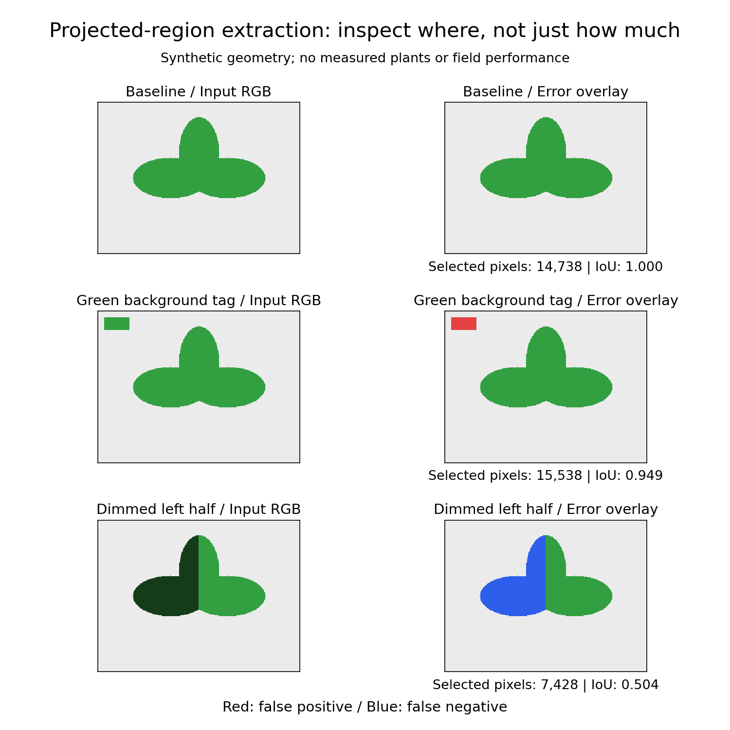
Red marks background selected as target; blue marks missed target pixels. Green regions retain their input colors. These are synthetic shapes, not plant photographs.
| Condition | Selected pixels | Plane-equivalent area [mm²] | IoU | Interpretation |
|---|---|---|---|---|
| clean | 14,738 | 3,684.50 | 1.000 | Matches synthetic reference |
| green_tag | 15,538 | 3,884.50 | 0.949 | Adds 800 background pixels |
| green_tag_roi | 14,738 | 3,684.50 | 1.000 | Excludes the tag in this layout |
| dim | 7,428 | 1,857.00 | 0.504 | Misses nearly half without changing shape |
| dim_lower_v | 14,738 | 3,684.50 | 1.000 | V minimum 40 recovers this dark region |
| wrong_scale | 14,738 | 5,305.68 | 1.000 | Correct mask, 44% larger conversion |
| clipped | 13,016 | 3,254.00 | 1.000 | Matches in-frame reference, but not the whole object |
The fixed green_tag_roi starts at (50,20), with width 230 and height 190 pixels. It was chosen to avoid this synthetic tag, not as a crop-independent region of interest. Growth beyond the ROI would exclude genuine target pixels.
Lowering minimum V is not a universal fix. It recovers the dim target here, but may admit dark green background in real scenes. Do not tune thresholds against the answers for each image and report accuracy only on those same images.
Evaluate area and location separately
For prediction P and reference G, intersection over union measures spatial overlap:
Equal numbers of extra and missed pixels produce zero area error despite incorrect locations. A reference [0,1,1,0] and prediction [1,1,0,0] each contain two selected pixels, but their IoU is 1/3.
Outputs also include precision, the correct fraction of selected pixels, and recall, the recovered fraction of reference pixels. mask_area_error_percent is pixel-count error against the reference, not physical error from scale calibration. It remains zero for wrong_scale. Undefined ratios, including the IoU of two empty masks, are JSON null rather than an assumed perfect score.
touches_frame flags selected pixels touching an image edge. It is true for clipped. It does not detect every incomplete object: segmentation might miss the edge pixels, or an internal ROI might remove part of the target. Inspect the image and ROI even when the flag is false.
Download and reproduce
Download the complete ZIP, Python source, expected results, README and manifest. The ZIP includes inputs, references, extracted masks and error overlays, all regenerable from the same source.
Tested environment: Linux x86_64, Python 3.12.3, NumPy 1.26.4 and OpenCV 4.6.0. Dependency versions are pinned for reproduction, not a certification of other operating systems or Python versions.
After extracting the ZIP, run:
python3 -m venv .venv
.venv/bin/python -m pip install -r requirements.txt
.venv/bin/python experiment.py --self-test
.venv/bin/python experiment.py --verify expected.json --out reproduced
On Windows, replace .venv/bin/python with .venv\Scripts\python.exe. The output directory must not exist; existing outputs are not overwritten. Results JSON and each condition's PNG files are saved. Baseline outputs are included under samples/.
Change the minimum V with:
.venv/bin/python experiment.py --min-v 40 --out lower-v
Only dim_lower_v always uses 40; other conditions use the supplied value. Changed results intentionally fail comparison with baseline expected.json. Do not expect baseline verification to pass after changing the experiment.
Seven tests cover a known rectangle, equal-area/different-location masks, empty masks, relationships among seven cases, invalid inputs, modified expected results and ROI omissions. The original download has no real-photo ingestion feature; the browser adapter is available above.
Evaluate on measured plants before making biological claims
The following is a proposed next-stage evaluation, not work completed by this synthetic example.
- Retain plant IDs, dates, illumination, camera geometry and original images.
- Define target membership, including whether stems or senescent leaves count, and create human reference masks.
- Separate threshold-development images from evaluation images. Consider splits by plant or acquisition date rather than merely separating adjacent video frames.
- Report errors by lighting, background, overlap and clipping, retaining area metrics, IoU and error overlays.
- To estimate actual leaf area or dry mass, collect corresponding independent reference measurements and validate that mapping as a separate model.
Time-series projected-area changes can result from posture or overlap. Producing an image metric does not establish growth rate or stress. First make the observation reproducible, then use reference data to test what it represents.
CEA root zone — separating EC, pH, oxygen and water balance
When the water level falls, what should be replaced?
A nutrient solution falls from 100 L to 90 L. That observation alone cannot distinguish evaporation, plant water uptake, leakage or drainage. It does not establish nutrient uptake either. Restoring volume and restoring nutrient composition are separate decisions.
Following the light environment guide, this article examines the root environment. It introduces a recirculating solution system; it is not a crop recipe or an automatic dosing implementation. All numerical examples are synthetic.
The root zone is the region where roots exchange water, nutrients and gases with their surroundings. A reservoir reading is useful, but need not describe the root surface, the end of a channel or the interior of a substrate.
Keep five measurements distinct
| Measurement | Meaning and units | What it does not establish alone |
|---|---|---|
| EC | Electrical conductivity, such as mS/cm | Individual nitrate, potassium or calcium concentrations |
| pH | Logarithmic quantity related to hydrogen-ion activity | Acid or base required to reach a target pH |
| Dissolved oxygen (DO) | mg/L or percent saturation | Oxygen delivery rate to the root surface |
| Water temperature | °C at the measurement location | Air temperature or the full root temperature distribution |
| Volume and flow | L and L/min, for example | Uptake of individual nutrients |
This is a measurement-planning table. Acceptable conditions depend on crop, growth stage and production system.
EC cannot reconstruct composition
1 mS/cm = 1,000 µS/cm = 1 dS/m. Record units. Conductivity also changes with liquid temperature: retain measured temperature, compensation settings and reference temperature, and distinguish compensated from uncompensated readings.
EC does not reveal individual salt concentrations, as explained in Oklahoma State University's water-test guide. A single reading cannot distinguish depletion of one nutrient from accumulation of another ion.
An EC-derived “ppm” display is also not a measurement of individual nutrients. Record its conversion factor and distinguish it from a laboratory concentration result. Use source-water and solution analysis when composition is needed.
OSU's nutrient-management guide identifies source-water testing, salt concentration, pH, alkalinity and nutrient ratios as relevant. Our operational inference is to avoid treating a return to the EC setpoint as proof that the original formulation has been restored.
Record pH and alkalinity separately
pH describes current acidity or basicity. Because it is logarithmic, a volume-weighted average of two pH readings generally does not give the mixed solution's pH. USGS: pH and Water
Alkalinity measures acid-neutralizing capacity. Two waters with the same initial pH can respond differently to the same acid addition when their alkalinity differs. USGS: Alkalinity and Water
A rule that always adds the same dose for a 0.5-unit pH error confuses these quantities. To evaluate an intervention, record source water, reservoir volume, substance and amount added, and the time of measurement after mixing. The water balance below cannot calculate the required dose.
Oxygen needs a delivery path
Equilibrium oxygen solubility depends on water temperature, atmospheric pressure and salinity. USGS DOTABLES uses these conditions to calculate solubility. At equal pressure and salinity, warmer water generally holds less dissolved oxygen at equilibrium. Check conversion conditions when comparing mg/L and percent saturation.
Roots require oxygen for respiration. Cornell's guide to hydroponic leafy greens discusses root oxygen supply and water temperature. An apparently adequate reservoir DO reading does not establish the same conditions inside a dense root mass. Record circulation, aeration and sampling location, including differences between the growing channel's inlet and outlet.
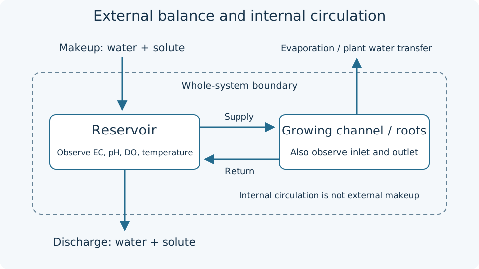
For a boundary enclosing the entire system, internal circulation is not an external water input. The diagram does not imply complete mixing or uniform oxygen.
With a substrate, water retention and air pathways also matter. Reservoir DO alone does not establish substrate aeration. Do not directly apply the single-liquid-compartment calculation below to the interior of a substrate.
Keep separate water and solute accounts
Choose a boundary enclosing the whole recirculating system, including reservoir, pipes and growing channels. Over one interval, let external additions be V_{in}, liquid discharge be V_{out}, and evaporation plus water transferred to plants be V_w, all in L.
Do not add internal pump circulation as makeup water. A reservoir-only boundary would instead count its outgoing and returning flows explicitly.
For one tracked solute, mass is M [mg] and concentration is C=M/V [mg/L]:
U is transfer to plants; R is net removal from the liquid phase, such as precipitation. Removal from the liquid does not mean destruction of matter. Liquid discharge carries both water and solute, unlike evaporation. For continuous discharge, use M_{out}=\int C_{out}(t)Q_{out}(t)dt to account for changing concentration.
The following original arithmetic example checks this bookkeeping. It is not a measured plant uptake rate, fertilizer recipe or EC prediction. Start with 100 L containing 10,000 mg of one component: 100 mg/L. Assume no additions or precipitation.
| Synthetic case | Final volume | Final solute mass | Final concentration |
|---|---|---|---|
| A: lose 10 L of water; solute remains | 90 L | 10,000 mg | 111.11 mg/L |
| B: transfer 10 L of water and 2,000 mg to plants | 90 L | 8,000 mg | 88.89 mg/L |
| C: discharge 10 L of uniform solution | 90 L | 9,000 mg | 100.00 mg/L |
The same volume decrease can accompany rising, falling or unchanged concentration. Adding 10 L of water containing none of the tracked solute restores A to 100 mg/L, but B reaches only 80 mg/L. Restoring volume does not restore solute mass.
Reproduce the comparison in Python
Save the following as root_zone.py and run python3 root_zone.py. Only Python's standard library is needed.
from math import isfinite


def concentration(volume_l, mass_mg):
    if not (isfinite(volume_l) and isfinite(mass_mg)):
        raise ValueError("finite values required")
    if volume_l <= 0 or mass_mg < 0:
        raise ValueError("positive volume and nonnegative mass required")
    return mass_mg / volume_l


initial_v, initial_m = 100.0, 10000.0
initial_c = concentration(initial_v, initial_m)
cases = {
    "A": (initial_v - 10, initial_m),
    "B": (initial_v - 10, initial_m - 2000),
    "C": (initial_v - 10, initial_m - 10 * initial_c),
}
for name, (volume, mass) in cases.items():
    print(f"{name}: {concentration(volume, mass):.2f} mg/L")
print(f"B + water: {concentration(cases['B'][0] + 10, cases['B'][1]):.2f} mg/L")
Outputs are 111.11, 88.89, 100.00 and 80.00 mg/L. Change the 2,000 mg removal in B to 1,000 mg: after the volume loss, concentration becomes 100 mg/L. Uptake can occur even when concentration is unchanged. Zero volume and negative remaining mass raise errors.
This code does not calculate EC, pH or DO. Correct bookkeeping for one component does not validate multicomponent chemical equilibrium or crop response.
Decide what to observe next
These are proposed observation combinations, not automatic dosing rules.
| Observation | Next checks |
|---|---|
| EC rises while volume falls | Makeup and discharge history, liquid temperature and compensation, water and solution composition |
| EC is stable while plant condition changes | Individual components, root-zone DO and temperature, flow, light and air history |
| pH changes again after adjustment | Mixing and measurement times, source-water alkalinity, addition history |
| Reservoir and outlet DO differ | Synchronized readings, sensor condition, circulation, aeration and root distribution |
Associate time, location, units and calibration with water volume, makeup, discharge and additions. Detailed sensor placement, individual nutrient management and dosing control are later steps. The foundation here is to distinguish an observed concentration from the mass remaining in the system.
Comments
Please log in to post a comment
No comments yet.