Contents — find the section you need
CEA nutrient tanks — accounting for replenishment and dilution
Restoring volume and concentration together
A tank holds 90 L at 80 mg/L of a tracked component. Adding 10 L of component-free water restores the volume to 100 L but reduces concentration to 72 mg/L. A low level and a component deficit therefore require separate accounting.
This guide extends root-zone foundations to discrete operations. All values are synthetic; 100 mg/L is an arithmetic target, not a crop recommendation. We track one component of known concentration, without calculating a fertilizer recipe, concentration from EC, or acid/base doses.
Define the boundary
Assume one perfectly mixed tank with crop-loop supply and return stopped. During each operation there is no uptake, evaporation, precipitation or reaction, and liquid volumes are additive. An operating tank needs supply and return volume and component flows in its balance. If the boundary encloses the entire circulating system, internal circulation is not external replenishment.
For volume V [L], concentration C [mg/L] and dissolved component mass M [mg], M=VC. Adding volume V_a at concentration C_a gives
Use C_a=0 only if the added water contains none of the tracked component. OSU's nutrient-management guide describes source-water analysis and attention to salt concentration, pH, alkalinity and nutrient ratios.
Compare three additions
Start with 90 L at 80 mg/L: 7,200 mg. Assume a stock concentration of 10,000 mg/L for this component.
| Operation | Final volume | Final component mass | Final concentration |
|---|---|---|---|
| Add 10 L of component-free water | 100 L | 7,200 mg | 72.00 mg/L |
| Add about 0.181818 L of stock only | About 90.181818 L | About 9,018.18 mg | 100.00 mg/L |
| Add 0.28 L of stock and 9.72 L of water | 100 L | 10,000 mg | 100.00 mg/L |
Stock also adds volume. For target concentration C_t, stock concentration C_s and stock volume x,
Raising concentration requires C_s>C_t>C_0. Stock at the target concentration cannot bring a lower initial concentration exactly to that target with a finite addition. A negative solution indicates that the proposed addition cannot meet the objective.
If final volume V_f is also prescribed and the makeup water contains none of the component,
Both additions must be nonnegative and the final volume must fit the vessel. Here they are 0.28 L of stock and 9.72 L of water. Specifying concentration alone gives a different answer from specifying both concentration and volume.
Draining and dilution have different effects
Now start with 100 L at 120 mg/L: 12,000 mg. Draining 10 L of well-mixed solution removes 1,200 mg. The remainder is 90 L and 10,800 mg, still at 120 mg/L. Adding 10 L of component-free water then gives 100 L at 108 mg/L.
Adding 20 L of water without draining instead gives 120 L at 100 mg/L. The tank still contains 12,000 mg, and it needs more spare capacity.
| Condition | Equation | Boundary |
|---|---|---|
| Drain D L first, then replace with water | C_1=C_0(1-D/V_0) | Perfect mixing; component-free refill |
| Add W L of water without draining | C_1=V_0C_0/(V_0+W) | Volume increases |
| Simultaneous inflow and outflow at constant volume | C(t)=C_{in}+(C_0-C_{in})e^{-Qt/V} | Perfect mixing, constant flow, no uptake or reaction |
For simultaneous replacement of 10 L, Qt/V=0.1 and C_{in}=0 give about 108.58 mg/L. This differs from the 108 mg/L obtained by draining first. Operation order belongs in the log.
Reproduce the accounting in Python
Save this as tank_accounting.py and run python3 tank_accounting.py. It uses only the standard library.
from math import isfinite


def mix(v, c, added_v, added_c):
    values = (v, c, added_v, added_c)
    if not all(isfinite(x) for x in values):
        raise ValueError("finite values required")
    if v <= 0 or min(c, added_v, added_c) < 0:
        raise ValueError("invalid volume or concentration")
    return (v * c + added_v * added_c) / (v + added_v)


v, c, target, stock = 90.0, 80.0, 100.0, 10000.0
x = v * (target - c) / (stock - target)
print(f"water top-up: {mix(v, c, 10, 0):.2f} mg/L")
print(f"stock addition: {x:.6f} L, {mix(v, c, x, stock):.2f} mg/L")
y = (100 * target - v * c) / stock
print(f"fixed final volume: stock {y:.2f} L, water {10-y:.2f} L")
print(f"drain then refill: {mix(90, 120, 10, 0):.2f} mg/L")
print(f"dilute only: {mix(100, 120, 20, 0):.2f} mg/L")
The outputs are 72.00 mg/L; 0.181818 L and 100.00 mg/L; 0.28 L and 9.72 L; 108.00 mg/L; and 100.00 mg/L. Before experimenting with another stock concentration, check the reachability conditions above and ensure the denominator is nonzero.
From accounting to control
OSU's irrigation-water test guide explains that EC and TDS do not identify individual salt concentrations. Substituting EC for C cannot calculate replenishment of a specific component. A mixed fertilizer changes several components at once, so meeting one target does not restore the entire composition.
A sensor also need not reach the perfectly mixed prediction immediately. OSU's nutrient-management guide calls for stirring and allowing readings to stabilize. Based on that distinction, this article proposes the following starting point for control design:
- Record the initial time, volume, sampling location, basis for component concentration, EC, liquid temperature and pH.
- Record stock composition, actual addition and drain volumes, and circulation state. Pump command duration alone does not establish actual flow.
- Wait for a mixing interval established on the equipment and stable measurements before reassessment. Avoid stacking additional commands in response to a local reading immediately after injection.
- Preserve prediction errors. Stop further additions to investigate abnormal levels, flow discrepancies or stale measurements. Establish tolerances and dose limits on the actual installation.
This is not a complete dosing-system specification. The worked examples validate arithmetic consistency of volume, component mass and concentration under stated assumptions. The next step is to connect commanded operations to observations using measured pump flow and mixing response.
CEA dosing pumps — volume calibration and mixing waits
Two checks before calling an addition “20 mL”
The tank-accounting guide calculated additions from water and component balances. A calculated 20 mL does not yet specify a pump run time. Finishing the injection also does not mean a tank reading is representative.
This guide separates command-to-volume calibration from checking when post-injection measurements can be reassessed. Every dataset below is an original synthetic example, not measured performance of a device or crop. The code does not operate equipment or calculate fertilizer recipes.
Hold calibration conditions constant
University of Georgia's fertilizer-injector guide explains periodic calibration and maintenance, operating flow ranges and pressure conditions. A water-proportional injector's ratio is different from the mL/s of a time-commanded pump considered here.
For a collection experiment, follow the equipment manual and record conditions consistently:
| Record | Purpose |
|---|---|
| Pump, speed setting, tubing, valves and service history | Identify the calibrated configuration |
| Liquid, temperature and density if used | Keep a water trial distinct from a stock-solution trial |
| Suction level, discharge elevation/pressure and plumbing | Preserve differences between collection and operation |
| Priming, bubbles and preceding idle time | Identify startup differences |
| Command start/stop, collection end and collected volume | Define whether post-stop dripping is included |
Disconnecting discharge plumbing for collection can change backpressure. An easy collection setup does not by itself establish delivery in the installed system. Keep preliminary water checks separate from confirmation with the intended liquid.
When weighing, convert net collected mass \Delta m [g] using liquid density \rho [g/mL]: V=\Delta m/\rho [mL]. Do not assume every liquid has a density of 1 g/mL. Record balance resolution, calibration status and timing accuracy.
A long-run average can misrepresent a short addition
Assume three trials at each duration, all starting in the same state.
| Command [s] | Three synthetic volumes [mL] | Mean [mL] |
|---|---|---|
| 10 | 15, 16, 17 | 16 |
| 20 | 35, 36, 37 | 36 |
| 30 | 55, 56, 57 | 56 |
| 60 | 115, 116, 117 | 116 |
The means follow V(t)=at+b=2t-4 [mL], with a in mL/s and b in mL. A 20 mL target gives (20-b)/a=12 s. Using the slope alone gives 10 s and just 16 mL in this example.
Using the 60 s average flow, 116/60 mL/s, instead gives approximately 10.34 s for 20 mL. The synthetic equation predicts about 16.69 mL at that duration. Which “flow rate” is used matters.
The −4 mL intercept is a regression coefficient over the sampled range, not proof of a physical two-second pure delay. Do not extrapolate outside 10–60 s, especially toward zero. For measured data, inspect residuals and consider a separate short-duration model if the relationship curves.
Each synthetic row has a sample standard deviation of 1 mL. Zero regression error on the means does not remove individual-shot variation. Three repeats also do not establish day-to-day variability or balance bias. Check measured predictions using additional durations and trials excluded from fitting.
Separate injection completion from mixing confirmation
OSU's nutrient-management guide calls for stirring and stable readings before assessment. Establishing a wait requires a post-injection time series distinct from the volume calibration.
Record synchronized measurements away from the injection point as well as nearby. Document volume, circulation flow, injection and sensor locations, temperature and sensor filtering. Mixing, transport and sensor response all contribute to the observed dynamics; one fitted response time is not automatically a pure mixing time.
For illustration, normalize a change from initial value y_0 to a known final value y_\infty:
Time zero is injection completion. This is a synthetic local measurement response, not a mass-conserving tank model. Assume time constants of 40 s and 80 s at locations A and B. Their continuous-time responses enter a 5% band around the final change after approximately 120 s and 240 s.
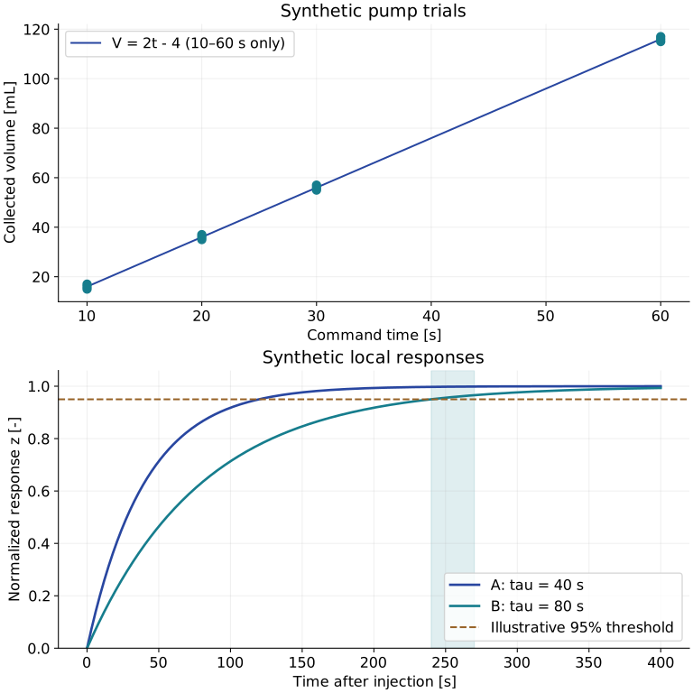
Top: three collected volumes per duration and the line fitted to their means. Bottom: synthetic responses A and B. Time is in seconds, volume in mL and normalized response is dimensionless. No measured data are shown.
Now impose an educational rule: with samples every 10 s, both locations must remain within 5% for 30 s before confirmation. B first qualifies at 240 s. The four samples at 240, 250, 260 and 270 s provide confirmation at 270 s. Checking A alone would qualify at 150 s and overlook B.
Neither 5% nor 30 s is a universal acceptance criterion. Choose criteria using measurement noise/accuracy, acceptable concentration deviation and sampling interval. Estimate final values independently, for example from sufficiently long records, and also inspect differences between the locations' final values. Normalizing each location separately can hide persistent spatial concentration differences. Do not use this normalization when the initial-to-final change is small relative to noise.
Reproduce the calculations
Save as pump_mixing.py and run python3 pump_mixing.py. Only the standard library is required.
from math import exp
from statistics import mean

# Synthetic data only; time [s], collected volume [mL].
runs = {10: [15, 16, 17], 20: [35, 36, 37],
        30: [55, 56, 57], 60: [115, 116, 117]}
ts = list(runs)
vs = [mean(runs[t]) for t in ts]
tm, vm = mean(ts), mean(vs)
a = sum((t-tm)*(v-vm) for t, v in zip(ts, vs)) / sum((t-tm)**2 for t in ts)
b = vm - a*tm
command = (20-b)/a
if not min(ts) <= command <= max(ts):
    raise ValueError("command outside calibration range")
print(f"fit: V = {a:.2f} t {b:+.2f}; 20 mL command = {command:.2f} s")
print(f"held-out 40 s: predicted {a*40+b:.2f} mL; reference 76.00 mL")

# Two synthetic normalized responses, sampled every 10 s.
# Four consecutive samples span 30 s. No missing samples here.
times = list(range(0, 401, 10))
errors = [max(exp(-t/40), exp(-t/80)) for t in times]
ready = next((times[i] for i in range(3, len(times))
              if all(e <= 0.05 for e in errors[i-3:i+1])), None)
print(f"two-location confirmation = {ready} s")
The outputs are slope 2.00, intercept −4.00, a 12.00 s command for 20 mL, 76.00 mL at 40 s, and confirmation at 270 s. The held-out 40 s reference also comes from the same synthetic equation, so it is not evidence of generalization to actual equipment. Changing the 80 s time constant to 120 s gives confirmation at 390 s. If no qualifying window exists in the recording, the code returns None.
Connect the checks to permission for another addition
A control implementation needs more than a timer. This article proposes separate stages for prechecks, one addition, mixing/measurement wait and reassessment. Out-of-range commands, missing or stale readings, stopped circulation, abnormal levels or failure to stabilize within the observation period should prevent further additions pending investigation. Do not fill missing samples with the previous value and count that as continuous stability.
An EC reading below target after waiting does not immediately establish a particular component deficit; preserve the distinction between EC and composition explained in root-zone foundations. The next step is to assess delivery predictions and waiting criteria against measured logs before designing dosing control with per-addition, cumulative and retry limits.
CEA dosing control — limits, measurement waits and fault states
A low reading does not justify repeated additions
Pump calibration and mixing waits separated delivered volume from the time at which observations settle. The next question is whether another addition is currently permitted. A low reading during mixing, an old sample or stopped circulation does not establish that permission.
This guide proposes an educational design with separate operating states and checks on volume, attempt count and observations. All values and inputs are synthetic, not operating limits or fertilizer recommendations. The Python example reproduces an authorization gate only; it does not operate a pump.
Calculate a candidate, then decide whether it may execute
A candidate derived from tank accounting still needs checks against the calibration range, equipment state and observations that can assess the previous operation.
UGA's injector guide explains periodic calibration and maintenance. OSU's nutrient-management guide calls for stirring and stable readings before assessment. The states and limits below are this article's proposed design, not a controller specification supplied by either source.
Separate six operating states
| State | Activity | Transition condition |
|---|---|---|
| CHECK | Validate observations, candidate, remaining budget and equipment | Record a reservation before DOSE; go to DONE if the objective is already met |
| DOSE | Issue one command for a unique operation ID | Confirm stopping before WAIT; timeout or flow mismatch leads to FAULT |
| WAIT | Prohibit new additions and collect post-stop observations | Qualifying observations lead to REVIEW; failure to settle by the deadline leads to FAULT |
| REVIEW | Reassess observations and history | DONE if satisfied, CHECK if another candidate is justified, FAULT for inconsistencies |
| DONE | Keep output stopped and close the record | A subsequent operation requires a new operating decision |
| FAULT | Request stopping and prohibit further additions | Explicit recovery after checking the cause, delivered amount and equipment |
Issuing a stop command is different from confirming that flow has stopped. Software state names cannot prevent a failed valve or pump. An implementation also needs output feedback, equipment-side stopping mechanisms and defined restart behavior.
Do not make FAULT automatically return to CHECK after a short wait. Repeating an operation without resolving its cause can accumulate unintended additions.
Charge the budget before issuing the command
Use illustrative limits of 16–20 mL per addition, 50 mL per operating session and at most three authorizations. The 16 mL minimum corresponds to the previous article's synthetic calibration at 10 s. These numbers are not equipment settings.
For already charged volume B [mL] and candidate d [mL], require
At authorization, record B\leftarrow B+d and n\leftarrow n+1 before proceeding to the command. This ledger represents consumed authorization capacity, not measured delivery. If communication fails immediately after a command, do not assume zero delivery and refund its capacity. Record measured and uncertain delivery separately.
| Synthetic operation | Candidate | Charged total after decision | Result |
|---|---|---|---|
| First | 16 mL | 16 mL | Allow |
| Second, after stopping, mixing and review | 16 mL | 32 mL | Allow |
| Third, after review | 18 mL | 50 mL | Allow |
| Fourth | 16 mL | 50 mL | Reject: attempt limit |
A 20 mL request after charging 32 mL is rejected because it would reach 52 mL, even with an attempt remaining. Reconsider observations and the candidate's basis instead of automatically clipping the dose to the remaining capacity.
Here a session is one correction sequence with a recorded start and finish. A loop iteration, page refresh or reconnection is not a new session. An operational system needs explicit budget renewal conditions, such as a defined time window or tank replacement, and records that survive restart. This example has no persistence.
Check freshness separately from stability
Receipt time alone does not establish freshness. Consider source measurement time, clock synchronization and order relative to the operation. Here age_s is an already converted measurement age accepted only between zero and five seconds. A negative age from a future timestamp is rejected too.
after_stop means the observation follows confirmation of the previous stop. For the initial addition, use an observation obtained after starting the current precheck. stable is an upstream decision based on a sequence of observations, as discussed in the previous guide. A single unchanging value does not establish stability: assess missing data, stuck sensors and disagreement between locations.
Five seconds is an educational assumption. A limit incompatible with the sampling interval and communication delay can reject useful observations. Simply increasing it does not solve stale-data problems.
Try the authorization gate in Python
Save as dosing_gate.py and run python3 dosing_gate.py. Only the standard library is required.
from math import isfinite


def gate(state, dose_ml, charged_ml, attempts, age_s,
         after_stop, stable, circulation, level_ok):
    """Offline authorization check; no hardware commands or persistence."""
    if state != "CHECK":
        return "STATE"
    if not all(isfinite(x) for x in (dose_ml, charged_ml, age_s)):
        return "INVALID"
    if charged_ml < 0 or type(attempts) is not int or attempts < 0:
        return "INVALID"
    if not all(type(x) is bool for x in
               (after_stop, stable, circulation, level_ok)):
        return "INVALID"
    if not circulation or not level_ok:
        return "INTERLOCK"
    if not 0 <= age_s <= 5 or not after_stop:
        return "STALE"
    if not stable:
        return "UNSTABLE"
    if not 16 <= dose_ml <= 20:
        return "DOSE_RANGE"
    if attempts >= 3:
        return "ATTEMPTS"
    if charged_ml + dose_ml > 50:
        return "BUDGET"
    return "ALLOW"


if __name__ == "__main__":
    charged, attempts, state = 0.0, 0, "CHECK"
    for requested in (16, 16, 18, 16):
        result = gate(state, requested, charged, attempts, 1,
                      True, True, True, True)
        if result == "ALLOW":
            # Charge BEFORE a simulated command; never refund uncertainty.
            charged += requested
            attempts += 1
            state = "WAIT"
        print(f"{requested} mL: {result}; charged={charged:.0f} mL")
        # Synthetic successful stop/mixing/reassessment, not a timer.
        state = "CHECK"
The first three decisions are ALLOW; the fourth is ATTEMPTS. Charged totals are 16, 32, 50 and 50 mL. Resetting the demonstration state to CHECK at the end of each iteration represents synthetic successful stopping, mixing and reassessment. An implementation must not execute that transition solely because a fixed timer expired.
This function is an offline educational gate with numeric arguments. It does not parse communication inputs, calculate a dose, establish stability, monitor actual flow or execute the state machine. It rejects NaN, infinity, negative charged volumes and invalid attempt counts, but is not a complete external-input API.
Exercise the rejection boundaries
| Input or situation | Expected result |
|---|---|
| Another candidate arrives in WAIT | STATE; no additional budget charge or command |
| Age is six seconds or negative | STALE |
| Observation precedes stopping, or is not stable | STALE or UNSTABLE |
| Circulation stopped or abnormal level | INTERLOCK |
| Candidate is 15 or 21 mL | DOSE_RANGE |
| Request 20 mL after charging 32 mL | BUDGET |
| Candidate or charged volume is NaN | INVALID |
An implementation must also test that resending an operation ID cannot execute twice. Commit budget changes and operation IDs together so competing requests cannot both spend the same remaining capacity. After interruption, reconcile persisted commands with actual equipment state before resuming.
What this establishes
The example checks authorization decisions against supplied inputs and bounds. It does not infer individual component deficits from EC or acid quantities from pH differences. It also does not validate growth, yield, equipment safety or concentration tracking.
The roles of accounting, delivery calibration, mixing assessment and authorization are now connected. Validation with measured equipment logs remains open. Next comes the water path through production systems such as NFT, DWC and drip, where the relationship between tank and roots changes.
Comments
Please log in to post a comment
No comments yet.