Contents — find the section you need
CEA production systems — water paths in NFT, DWC and drip
The same solution takes different paths to the roots
Setting tank EC, pH and temperature does not establish uniform conditions around every root. A thin moving film, an immersed root system and a drip-fed substrate store and transport water differently, changing both observation locations and accounting boundaries.
Following dosing authorization, this guide compares NFT, DWC and substrate drip. The aim is to trace water from the tank to roots and then to return or discharge, not rank systems or recommend equipment. All numerical examples are synthetic.
Distinguish the three root environments
| System | Root environment | Main water path | Quantities to distinguish |
|---|---|---|---|
| NFT: Nutrient Film Technique | Roots in a channel with a thin nutrient film | Tank → distribution → channels → collection → tank | Per-channel flow, return and local pooling |
| DWC: Deep Water Culture | Roots immersed in a production pond or vessel | Circulation within or between connected vessels; oxygenation also managed | Volume, circulation distribution, root-zone DO and temperature |
| Substrate drip | A medium containing solids, water and air | Tank → emitters → substrate → drainage | Per-plant application, storage change and drainage |
NFT structure follows Virginia Cooperative Extension's NFT guide; the DWC pond, circulation and oxygenation follow its DWC guide. The University of Kentucky's hydroponic irrigation guide describes drip delivery to individual containers and media.
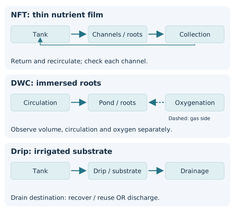
Simplified representative paths, not a plumbing specification. Drain recovery and external discharge are alternative configurations, not necessarily simultaneous flows.
NFT: inspect distribution, not just pump flow
NFT feeds root-bearing channels and collects their downstream return. A running pump does not establish that each channel is unobstructed or receives an appropriate share. Local pooling can also occur. This article therefore proposes combining pump status with observations of individual channel inlets and outlets.
VCE's NFT guide describes drainage-supporting structures, collection plumbing and pump sizing that accounts for lift and friction. Check flow paths after roots develop as well as in empty channels.
In a synthetic example, eight channels each receive 1 L/min for 60 minutes: 480 L of accumulated circulation. An independently specified 3 L of external makeup during the same interval is compatible with that circulation. The same water can pass repeatedly, so 480 L is not an external water-use total.
Water can also drain back from channels and pipes after pump shutdown. Do not attribute the entire running-versus-stopped tank-level difference to plant uptake or transpiration. Separate a tank-only balance from a boundary enclosing plumbing and production vessels.
DWC: retained water does not establish oxygen delivery
DWC roots are immersed in solution, unlike the thin-film configuration. A large liquid volume alone does not ensure oxygen delivery. VCE's DWC guide describes circulation and oxygenation arrangements using a venturi or air pump and diffuser.
From that distinction, this article proposes logging DO and temperature at several locations, including dense root regions, together with liquid level. Record whether circulation and aeration share equipment or are independent. Air flow and water flow can both use L/min, but they are different balance terms.
For a 200 L vessel recirculated at 10 L/min, nominal turnover is
This does not mean every parcel passes exactly once in 20 minutes. Short-circuit flow and stagnant regions alter the distribution. It is neither fresh-water replacement time, mixing wait time, nor the time needed for adequate oxygenation.
If circulation or aeration stops, retained water does not establish maintained root conditions. This ratio cannot predict an allowable outage duration.
Drip: account for water retained in the substrate
Drip describes delivery, not necessarily disposal. Distinguish recovery/reuse from discharge outside the system. Kentucky's guide discusses drip-fed Bato/Dutch buckets and bag/container systems with collected drainage.
Some applied water remains in the substrate at the end of the observation interval. For a boundary around the substrates, let I be applied water, D drainage, \Delta S the change in retained water, U transfer into plants, E evaporation and L other unmeasured outflow. All are in litres over the same interval:
Consequently, I-D alone is not plant water uptake. When estimating storage changes by weighing, define how changes in plant mass, containers and other non-water contributions are handled.
In a synthetic example, eight emitters each deliver 0.05 L/min for a total of ten operating minutes, applying 4 L. Across the same two-hour observation window containing that operation, drainage is 1 L and substrate water storage rises by 0.5 L. The residual is 4-1-0.5=2.5 L. This represents U+E+L, not plant uptake alone.
Drainage divided by application is 25% for that window. Cutting collection short changes the result, so align the numerator and denominator intervals. The 25% value is an arithmetic outcome, not an irrigation target.
Keep the three quantities separate in Python
Save as system_water_paths.py and run python3 system_water_paths.py.
# Synthetic arithmetic only: not crop or equipment recommendations.
channels, flow_l_min, minutes = 8, 1.0, 60
circulated_l = channels * flow_l_min * minutes
makeup_l = 3.0  # Independently specified external addition.
print(f"NFT: circulated={circulated_l:.1f} L; makeup={makeup_l:.1f} L")

pond_l, recirculation_l_min = 200.0, 10.0
print(f"DWC: nominal turnover={pond_l / recirculation_l_min:.1f} min")

emitters, emitter_l_min, on_minutes = 8, 0.05, 10
irrigation_l = emitters * emitter_l_min * on_minutes
# Drainage and storage change measured over the SAME two-hour window.
drain_l, storage_change_l = 1.0, 0.5
residual_l = irrigation_l - drain_l - storage_change_l
print(f"Drip: applied={irrigation_l:.1f} L; residual={residual_l:.1f} L")
print(f"Drain/applied={100 * drain_l / irrigation_l:.1f}%")
Outputs are 480 L circulated and 3 L makeup for NFT; 20 minutes nominal turnover for DWC; and 4 L applied, 2.5 L residual and 25% drainage/application for drip. These are independent examples, not a water-efficiency experiment comparing production systems.
Bring the physical paths back into control
The following observation plan is derived from this article's accounting boundaries. Include system-specific paths alongside shared EC and pH settings.
| System | Check before additional action | Insufficient by itself |
|---|---|---|
| NFT | Distribution and return flow, pooling and leaks | Pump ON or tank EC |
| DWC | Root-zone DO/temperature distribution, circulation and oxygenation | Water present or nominal turnover |
| Drip | Emitter variability, substrate water status, drainage quantity and destination | Total pump flow or tank level |
If return solution is reused, record its quantity, quality and treatment path. Equal EC does not make return solution equivalent to source water. Detailed sanitation and treatment design require separate work.
This guide establishes water paths and measurement boundaries for three systems. Aeroponics, multi-tier distribution and return, and measured control validation remain open. Next comes the relationship between lift, flow distribution and drainage as height and branching increase in multi-tier cultivation.
CEA multi-tier water delivery — head, branch flow and drainback
A running pump does not establish equal flow to every tier
Extending production water paths vertically introduces lift, branch resistance and shutdown drainback. Flow to one tier can be inadequate while other branches keep the total looking substantial.
This guide considers an open low reservoir feeding atmospheric outlets at several heights, with gravity collection. A synthetic pump curve and branch model illustrate the relationships. They do not select equipment, crop flow requirements, pressure-compensating emitters or misting nozzles.
Head is more than rack height
NDSU's irrigation-pump guide distinguishes static, pressure, friction and velocity head and relates flow/head requirements to pump curves. Between a source free surface and an outlet, the general accounting is
All terms are metres. Elevation difference is \Delta z, pressure difference is \Delta p, and h_L includes pipe, fitting and valve losses. Maximum head at no flow is different from available head at a required flow. Maximum flow and maximum head are not simultaneous operating capabilities.
VCE's NFT guide describes lift/friction requirements and gravity collection. Where pressure is released into open channels, the descending return does not simply cancel the lift. That boundary differs from a continuously full closed loop.
Solve the three branches together
Take the reservoir free surface as elevation zero. Let H be available head at an ideal manifold at that elevation, approximating pressure head and neglecting velocity-head differences within the manifold. Branch outlets are atmospheric; outlet velocity effects are included in the simplified quadratic resistance.
Use the synthetic pump curve H_p(Q)=6-0.020Q^2 and common-pipe loss 0.005Q^2. Flow Q is in L/min and head in metres, so the coefficients use m/(L/min)². Do not transfer them unchanged to a formula using m³/s.
For outlet elevation z_i [m] and resistance coefficient k_i,
must hold together. Branches are assumed not to reverse flow: insufficient head gives q_i=0. This does not model startup air removal or siphoning.
| Synthetic case | Elevations z_1,z_2,z_3 [m] | Resistance k_1,k_2,k_3 [m/(L/min)²] |
|---|---|---|
| A: baseline | 1, 2, 3 | 0.5, 0.5, 0.5 |
| B: increased upper resistance | 1, 2, 3 | 0.5, 0.5, 2.0 |
| C: raised upper outlet | 1, 2, 7 | 0.5, 0.5, 0.5 |
Equal branch resistance does not give equal flow when elevations differ. Case B abstracts increased resistance, such as an obstruction; it does not predict an actual clog geometry.
Changes hidden by total flow
| Case | Manifold H [m] | Lower [L/min] | Middle [L/min] | Upper [L/min] | Total [L/min] |
|---|---|---|---|---|---|
| A | 4.778 | 2.749 | 2.357 | 1.886 | 6.992 |
| B | 5.011 | 2.832 | 2.454 | 1.003 | 6.289 |
| C | 5.253 | 2.916 | 2.551 | 0.000 | 5.467 |
In B, upper-tier flow nearly halves while lower and middle flows increase. Reduced common flow changes the manifold head through both the pump curve and common-pipe loss. Adjusting one branch does not leave the others unchanged.
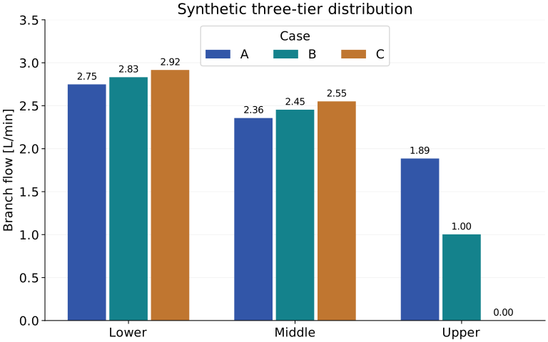
Horizontal axis: lower, middle and upper tiers. Vertical axis: L/min. All bars are synthetic model outputs, not measurements.
C retains total flow but does not supply the upper tier. Finding a numerical solution is different from serving every tier. Even positive flow needs comparison against the actual crop requirement.
OSU's pump-system testing guide distinguishes system and pump performance curves. Building on that distinction, this article proposes recording branch flows, manifold pressure and reservoir level alongside total flow. Plumbing changes and a falling reservoir level can change the operating point.
Reproduce distribution and drainback in Python
Save as multitier_flow.py and run python3 multitier_flow.py. Only the standard library is required. Bisection finds the zero of a monotonic residual for these synthetic equations; this is not general-purpose pipe-design software.
from math import sqrt, isfinite


def solve(heights, resistance):
    # Synthetic steady model: head [m], flow [L/min].
    if not heights or len(heights) != len(resistance):
        raise ValueError("matching nonempty branches required")
    if any(not isfinite(z) or z < 0 for z in heights):
        raise ValueError("finite nonnegative heights required")
    if any(not isfinite(k) or k <= 0 for k in resistance):
        raise ValueError("finite positive resistance required")
    lo, hi = 0.0, 6.0
    for _ in range(80):
        h = (lo + hi) / 2
        flows = [sqrt(max(h-z, 0)/k)
                 for z, k in zip(heights, resistance)]
        if h + 0.025 * sum(flows)**2 > 6:
            hi = h
        else:
            lo = h
    h = (lo + hi) / 2
    flows = [sqrt(max(h-z, 0)/k)
             for z, k in zip(heights, resistance)]
    return h, flows


if __name__ == "__main__":
    cases = {"A": ([1, 2, 3], [0.5, 0.5, 0.5]),
             "B": ([1, 2, 3], [0.5, 0.5, 2.0]),
             "C": ([1, 2, 7], [0.5, 0.5, 0.5])}
    for name, (z, k) in cases.items():
        h, flows = solve(z, k)
        print(name, f"H={h:.3f} m", [round(q, 3) for q in flows],
              f"total={sum(flows):.3f} L/min")
    drainback_l = 12 * 1.5 * 0.08 * 0.005 * 1000 + 2.8
    print(f"drainback={drainback_l:.1f} L; free-space shortfall={drainback_l-8:.1f} L")
The outputs match the table. H is manifold head after common-pipe loss, not pump head itself. In A, pump head is approximately 5.022 m while manifold head is approximately 4.778 m.
The model assumes steady conditions, fixed reservoir level and constant resistance. It excludes suction conditions, cavitation, equipment efficiency, water hammer, trapped air and resistance changes as roots develop. Actual equipment requires separate checks against manufacturer curves and suction conditions.
Provide space for returning water after shutdown
Supply capacity is only one check. The reservoir must also accept drainback after stopping. Drainage depends on slope, section, air paths, obstruction and outlet submergence, not just supply-pump flow.
In a separate synthetic example, twelve channels each contain water over 1.5 m length, 0.08 m wetted width and 0.005 m average depth. Assume all of it returns: 7.2 L from channels plus 2.8 L from pipes gives 10 L. Root displacement and detailed geometry are ignored in this arithmetic example.
If the running reservoir has 8 L of free space, the calculated shortfall is 2 L. Compare against space above the operating level, not total tank capacity. Ten litres of free space is not a validated design allowance; actual drainback, local overflow and measurement uncertainty still need assessment.
Adequate reservoir space also does not prevent an upstream collector from overflowing when blocked. Record shutdown drainback and running drainage capacity as separate checks.
Observations added by multiple tiers
| Situation | Record | Distinction |
|---|---|---|
| Normal operation | Total/branch flows, pressure and level | Supply capability versus distribution |
| After a branch adjustment | Changes at every tier | Interaction between branches |
| Stop and restart | Drainback, maximum level and flow recovery | Free space and startup supply |
| After root development | Pooling, drainage and flow paths | Initial versus operating resistance |
The input to dosing authorization should establish supply to the required tiers and successful return, beyond a pump-ON signal. This guide establishes a synthetic model and observation plan; it does not validate pipe sizes or crop performance. Next comes aeroponics: the path to misted roots and the roles of nozzles, pressure and spray intervals.
CEA aeroponics — separate mist paths, pressure and intervals
Wet roots do not prove a functioning spray system
The multi-tier guide showed how elevation and branch resistance change flow. Aeroponics delivers droplets rather than a continuous film. A running pump does not establish root delivery when pressure, clogging, droplet reach or post-stop repressurization has not been checked.
This guide defines observation boundaries for a mist system. It does not recommend nozzle models or crop-specific intervals. Values are synthetic.
Separate four parts of the path
| Part | Record | It does not establish |
|---|---|---|
| Tank and suction | Level, temperature, strainer differential | Nozzle-tip pressure |
| Pump and piping | Flow, discharge pressure, power and pulsation | Droplet distribution at each nozzle |
| Nozzle row | Inlet pressure, nozzle collection volumes and clogs | Wetness at the root surface |
| Root chamber and drain | Root positions, recovered liquid and leaks | Water status before the next spray |
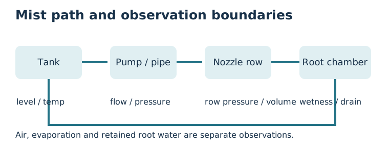
Arrows show a representative liquid path. Air movement, evaporation and liquid retained on roots are separate observations.
Do not substitute pump outlet pressure for nozzle pressure
Outlet pressure changes across branches, filters, elevation, fittings and nozzles. If equal nozzle delivery is an assumption, record row inlet and end pressure together with collection volume by nozzle.
Use the synthetic relation q_i=k_i\sqrt{\max(p_i-p_{min},0)}, where p is kPa, q is mL/min and k_i is a synthetic coefficient. This is not a manufacturer curve; it only illustrates reduced delivery below available pressure.
Different k_i values produce different flow at the same pressure. Recalibrate after changing a nozzle while preserving the actual row configuration. Parallel rows can change pressure and flow in the other rows when one nozzle clogs.
An interval is more than a timer
A setting of 10 seconds on and 50 seconds off says nothing about retained water, droplet reach, temperature, humidity or drain return. Record these timestamps separately:
- Command start and actual pump start.
- Nozzle-row pressure reaching its operating value.
- First spray arrival in the root chamber.
- Command stop and confirmed zero flow.
- The observation time at which another spray is permitted.
Do not treat a stop message as confirmed zero flow. As in dosing authorization, hold faults rather than stacking retries and recover explicitly after checking the cause.
Calculate a synthetic nozzle row
Give three nozzles 120 kPa inlet pressure, a 40 kPa minimum operating pressure and coefficients [2.0, 1.8, 1.2]. Equal command time does not imply equal nozzle volume.
from math import sqrt

pressure_kpa = 120.0
minimum_kpa = 40.0
coefficients = [2.0, 1.8, 1.2]
flows = [k * sqrt(max(pressure_kpa - minimum_kpa, 0))
         for k in coefficients]
print([round(q, 1) for q in flows])
print(round(sum(flows), 1))
print(f"10 s spray volume = {sum(flows) / 6:.1f} mL")
The output is [17.9, 16.1, 10.7], 44.7 mL/min and 7.5 mL in 10 seconds. The point is to preserve coefficients, pressure and per-nozzle variation, not to recommend these values.
Keep permission and fault conditions separate
| Situation | Check | Why not spray again immediately |
|---|---|---|
| Low end pressure | Filter differential, level and leaks | Extending runtime can overfeed another branch |
| One nozzle low | Clog and pre/post replacement collection | It may not be a chamber-wide deficit |
| Dripping after stop | Valve closure, residual liquid and check valve | Command time no longer equals delivered volume |
| Missing root-chamber observation | Sensor timestamp, camera and recovery | Old data cannot justify a shorter interval |
Do not treat spray volume, droplet distribution, root-surface retention and recovered liquid as one variable. A wet observation at one point cannot establish every nozzle.
Scope
This guide covers liquid paths, pressure observations and interval timestamps. Nozzle selection, droplet-size measurement, sanitation, outage backup and measured root-water response remain open. The next step is the sanitation and reuse boundary for recovered solution across these systems.
Comments
Please log in to post a comment
No comments yet.