Contents — find the section you need
A supply deficit pushes the frequency of an operating synchronous grid downward. Complete loss of voltage in a blackout is not the same as a slowly declining frequency. This educational model assumes continued energization and represents one area by a single frequency.
Separate inertia from corrective response
Inertia affects the rate of change; primary response changes power to counter the deficit. Inertia alone does not remove it. Background is available in the grid-inertia introduction and the 2020 Inertia and the Power Grid overview. All numbers below come from our stated assumptions, not real grid-event measurements.
Equations and units
Let f₀=50 Hz and x=(f−f₀)/f₀. Additional generation p and demand increase/supply loss d are per-unit values on the same power base:
H is inertia constant [s], D frequency-sensitive load response, R droop and Tg governor-response time constant [s]. Use D=1, R=0.05 and Tg=0.5 s. R=0.05 means a steady −0.05 pu frequency deviation requests +1 pu generation. Headroom, saturation and deadband are omitted.
Without primary response, replace −x/R in the second equation by zero. D remains, so this is not a system without all response. Start with x=0 and p=0; step d to 0.05 at 2 s.
Reproduce the calculation
Save the script and run python3 engineering_labs.py. Execution was checked with Python 3.12.3, NumPy 1.26.4 and Matplotlib 3.6.3. Fourth-order Runge–Kutta integrates 0–30 s with a 0.01 s step. Halving the step to 0.005 s changes results by at most about 1.8×10⁻⁹ Hz. That checks discretization, not physical model validity.
The CSV includes time and four frequency curves. The summary records minimum, endpoint and initial rate.
Read the results
| H [s] | Primary response | Initial RoCoF [Hz/s] | Minimum over 0–30 s [Hz] | Frequency at 30 s [Hz] |
|---|---|---|---|---|
| 2 | No | −0.625 | 47.502 | 47.502 |
| 5 | No | −0.250 | 47.652 | 47.652 |
| 2 | Yes | −0.625 | 49.786 | 49.881 |
| 5 | Yes | −0.250 | 49.846 | 49.881 |
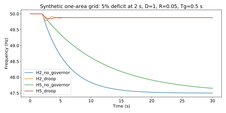
Immediately after the disturbance, p and x are still zero, giving initial RoCoF −f₀d/(2H). Greater H slows the initial drop. Primary response recovers from the nadir but does not restore exactly 50 Hz.
Verify the steady offset analytically
Set derivatives to zero with primary response:
H does not appear in this steady-state equation. Distinguish changing inertia from secondary control restoring nominal frequency. Without primary response, the model tends to 47.5 Hz; the H=5 case is still approaching that value at 30 s.
Limits and next experiment
Voltage, spatial network differences, loss of synchronism, protection, load shedding and storage limits are omitted. Curves reaching the 47 Hz range are formal linear-model outputs, not a prediction that real grids continue operating there without protection.
First fix H and change only R or Tg. Then cap generation response to distinguish faster response from available headroom. The power learning guide connects this model to transmission and storage foundations.
Comments
Please log in to post a comment
No comments yet.