Contents — find the section you need
Change parameters and verify
Open the panel, then press Run to load Python. You can stop execution and reset parameters. Results are computed on this device. No Python installation is required.
Local execution steps below are optional for reproducing the source results; they are not required for the browser experiment.
The experiment controls are in English.
Explore current coordinates and electrical angle
The panel above is a one-instant coordinate exercise. Supply actual current components in the true rotor frame, mechanical angle, pole-pair count, an electrical-angle error, and a hypothetical torque constant. It constructs balanced phase currents and transforms them back using the supplied estimated angle. These are imposed currents, not current references tracked by a controller. No motor, inverter or local Python is required.
The convention is explicit: α aligns with phase a; β is +90° counterclockwise from α. The true d axis follows rotor flux at θe=p θm, with fixed zero offset 0; q leads d by +90°. Positive angles are counterclockwise. p counts pole pairs, not poles. The display includes unwrapped electrical angle and its modulo-360° direction. Four pole pairs and 90° mechanical angle give 360° electrical angle, equivalent to 0° for the transforms. Changing p here changes the angle mapping only; the separately supplied torque constant stays fixed.
We use amplitude-invariant Clarke normalization with zero sequence fixed to zero. With R(θ)=[[cosθ,−sinθ],[sinθ,cosθ]], first form [iα,iβ]=R(θe)[id,iq]. Generate ia=iα, ib=−iα/2+√3 iβ/2, ic=−iα/2−√3 iβ/2. Thus ia+ib+ic=0. Clarke recovers iα=(2/3)(ia−ib/2−ic/2) and iβ=(ib−ic)/√3. These are instantaneous signed amperes, not phase RMS values. This amplitude normalization is not power invariant: ia²+ib²+ic²=(3/2)(id²+iq²).
The estimated angle is θ̂e=θe+Δθe. Park computes [id̂,iq̂]=R(θ̂e)ᵀ[iα,iβ]. Consequently id̂=id cosΔ+iq sinΔ and iq̂=−id sinΔ+iq cosΔ. At true id=0, iq=3 A and error +90°, the displayed estimated components become id̂=3 A, iq̂≈0. The original phase currents stay the same when only this angle error changes. The diagram shows the same stationary current vector with true and estimated axes; axis-arrow lengths are illustrative and do not encode current. All current scales are shared across A/B.
The inverse uses the same estimated angle: [iα′,iβ′]=R(θ̂e)[id̂,iq̂], then the same inverse Clarke equations. The maximum absolute reconstructed-phase difference should be small even at an incorrect angle. This residual measures algebraic consistency and floating-point roundoff; it cannot establish encoder alignment, sensor accuracy or a working FOC loop. Presets compare +/−90° errors, 180° error, mixed d/q current, zero current, negative q current, and electrical-angle wrapping. A zero vector hides every angle error.
A separate simplified nonsalient PMSM relation gives Te=Kt × true iq. Default Kt=0.10 N m/A and iq=3 A give 0.30 N m. Kt is defined for this amplitude-invariant peak-dq convention and includes the motor-specific conversion; it is not a phase-RMS constant to substitute blindly. The model omits reluctance torque and assumes constant flux. Angle error changes the displayed components but does not change imposed current or modeled torque. A real feedback loop using the wrong angle may change currents; that behavior is not simulated. Nonzero d current is a coordinate example, not a field-weakening or current-limit recommendation.
No PI control, PWM, DC-bus limits, voltage equations, speed dynamics, saliency, field weakening, sensor noise, heating, protection or hardware operation is modeled. Inputs are synthetic teaching assumptions. Use the separate PID Lab for controller behavior and the reducer Lab for mechanical transmission arithmetic.
Reference reviewed 2026-09-20: TI PMSM FOC report, sections 4–5. This exercise states its normalization and sign convention directly; it does not reproduce the report's motor-control implementation.
驱动器无法直接设定机械转速。它产生电压,改变绕组电流和磁场,然后产生转矩,进而改变电机的旋转。磁场定向控制 (FOC) 使用与旋转磁场对齐的坐标系来简化电流控制。本介绍重点关注永磁同步电机 (PMSM)。
电流、转矩和转速分离
简化的机械方程为:
J 为惯性矩 [kg·m²],ω 为机械角速度 [rad/s],Te 为电磁转矩 [N·m],TL 为负载转矩 [N·m],B 为粘性阻力 [N·m·s/rad]。在较大的惯性或负载下,较大的转矩并不一定需要立即改变转速。保持恒定转速也需要转矩。
外环速度控制,内环电流控制
转速误差驱动 PI 控制器产生与转矩相关的电流参考值。内环电流 PI 控制器生成电压参考值;PWM 通过逆变器开关实现这些电压参考值。
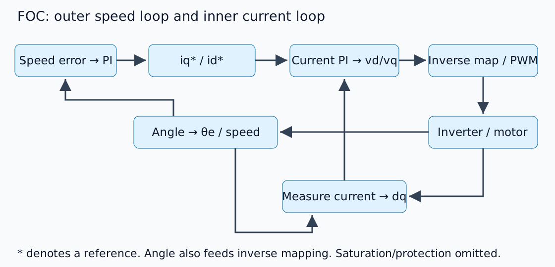
星号表示参考文献。外环设计假设电流跟踪响应足够灵敏,但任何通用的带宽比都无法忽略被控对象的动态特性和延迟。TI PMSM FOC报告的第4-5节解释了变换和基本结构。这是一张原始的解释性示意图,并非产品电路图。
在旋转坐标系中查看三相
克拉克变换将相电流映射到固定的αβ轴;帕克变换将其旋转到与转子磁链对齐的dq轴。d轴跟随磁链,q轴垂直于d轴。这假设平衡相中的零序可忽略不计,并且幅值/功率归一化一致。
对于低速的简化表面磁电机,适当定义的转矩常数允许Te≈Kt iq。假设 Kt=0.10 N·m/A 且 iq=3 A,则可得 0.30 N·m。这是在明确约定下的算术运算,并非允许随意替换相均方根电流。请将制造商提供的常数与 dq 变换定义进行匹配。
电角度与机械角度不同
对于 p 对极,电角度为:
四对极将 90° 的机械运动转换为 360° 的电运动。编码器方向反转、零点偏移错误或极点与极对混淆都会导致测量电流旋转到错误的轴上。调谐前,请检查角度、相序和电流传感器符号/偏移。
id=0 并非适用于所有工作条件
一个基本示例通常会将 d 轴参考设置为零。内部磁体凸极效应、最大转矩/安培运行和高速弱磁需要其他参考。增加反电动势也能防止电流在直流母线电压范围内跟踪。
电流和电压限制是不同的。积分通过饱和状态会延迟恢复,因此需要防饱和设计。未能达到目标转速并不一定意味着速度增益不足。
实施前的检查
本文是对控制结构的解释,而非逆变器实测。实际应用必须考虑电流采样时序、PWM 同步、角度延迟以及保护/停止条件。在硬件通电之前,请将已知的矢量和角度输入到 dq 变换和逆变换中,并验证往返行程。
评论
请先登录。
暂无数据。