Contents — find the section you need
Background and reading guide
Background Basic probability and machine learning.
Fundamentals · Explanations of principles, structure and trade-offs.
The basics of reinforcement learning and Q-learning and DQN, covered so far, assumed an MDP in which the environment reacts to only a single agent. But there are plenty of settings where multiple agents act on the environment at the same time — multiple transport robots in a warehouse, competitive games, a swarm of drones sharing communication duties. Multi-Agent Reinforcement Learning (MARL) deals with a difficulty that doesn't exist in single-agent RL: in this setting, everyone besides you is also learning, and keeps changing.
The 30-Second Summary
- In a single-agent MDP, the environment's transition probability P(s'\mid s,a) is fixed, but in a multi-agent environment where other agents are also learning and changing their policies, what one particular agent sees as "the environment" changes over time — this is called non-stationarity.
- Settings broadly split into cooperative (everyone maximizes a shared reward), competitive (zero-sum-like, beating an opponent), and mixed (partly cooperative, partly competitive), and the required algorithm changes accordingly.
- CTDE (Centralized Training with Decentralized Execution) — where learning uses global information but execution has each agent act on its own observations alone — is the mainstream framework that's practical for real hardware and real environments.
- How to distribute a shared reward across individual agents' contributions — the credit assignment problem — is the single biggest technical challenge in cooperative MARL.
- MADDPG (Lowe et al., 2017) and QMIX (Rashid et al., 2018) are representative algorithms that concretize CTDE, from the standpoint of Actor-Critic and Q-value factorization respectively.
1. Why Does the Single-Agent Framework Break Down?
The MDP's central assumption was that the environment's transition P(s'\mid s,a) and reward R(s,a,s') are fixed, independent of the agent's policy. Even as the agent updates its policy, the physical laws of the environment itself don't change.
In an environment with multiple agents, this premise breaks down. What agent i sees as "the environment" now includes not just physical law but the policies \pi_{-i} of the other agents -i (everyone besides i). Because the other agents are also learning simultaneously and continually updating \pi_{-i}, the effective transition probability that agent i experiences,
changes every time \pi_{-i} changes. This is non-stationarity. From agent i's perspective, an action that worked well yesterday might not work today, now that the other side's policy has changed. Even storing old transitions in a replay buffer can be actively misleading — that experience was gathered against an opponent who "no longer exists."
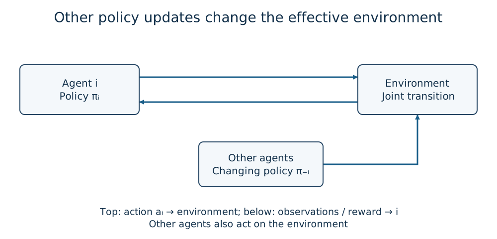
Figure 1 — What "the environment" is for agent i includes not just physical law but the other agents' policies. As long as the others keep learning, the transition distribution i experiences keeps moving.
2. Cooperative, Competitive, and Mixed: Reward Structure Shapes the Problem
The character of a multi-agent problem shifts dramatically depending on how reward is assigned.
| Setting | Reward Relationship | Representative Example | Main Difficulty |
|---|---|---|---|
| Cooperative | Everyone maximizes a common or highly correlated reward | Multiple warehouse robots maximizing transport efficiency | Credit assignment, communication design |
| Competitive | One side's gain is the other's loss (near zero-sum) | Competitive games, price-competition simulations | Must track the opponent's adaptation, unstable equilibria |
| Mixed / general-sum | Partly cooperative, partly adversarial | Multiple vehicles at an intersection, cooperative robots competing for a resource | Switching between situations calling for cooperation and situations calling for competition |
Cooperative settings are often formalized mathematically as a Dec-POMDP (Decentralized Partially Observable MDP), where everyone aims for the same set of optimal policies. Competitive settings are evaluated using concepts close to Nash equilibrium in game theory, where a single "optimal policy" may not even exist — because as the opponent's policy changes, what's optimal for you changes too. Mixed settings are the closest to reality, but come with the fewest theoretical guarantees.
3. CTDE: Centralized Training, Execution Left to the Field
CTDE (Centralized Training with Decentralized Execution) is widely used to deal with non-stationarity. During training (inside a simulator, or during an offline training phase), you're allowed to use central information that sees every agent's observations, actions, and sometimes rewards, all at once. But at execution time (on real hardware, in a production environment), each agent decides its action using only the local observation from its own sensors.
The practical reason CTDE works is clear. Given communication bandwidth and latency constraints, it's often unrealistic for a real fleet of robots or drones to operate while constantly sharing every agent's state. But inside a simulator or a training server, you can use all the information without worrying about communication cost. CTDE is a design that makes maximum use of this "privileged information available only during training," while still leaving behind a policy that can act autonomously at execution time.
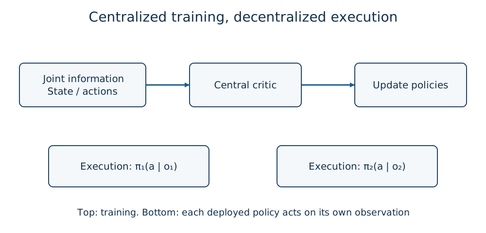
Figure 2 — During training, a central critic (or mixing network) integrates everyone's information; at execution time, each agent decides based on local observation alone. Separating the two lets non-stationarity be absorbed on the training side while tolerating execution-time communication constraints.
4. The Credit Assignment Problem: Whose Success, Whose Failure
In a cooperative setting, when all you get is a single shared reward r, it's not self-evident which of n agents' actions actually contributed to that reward. Give every agent the same reward as-is, and an agent that was actually slacking off receives just as "good" an evaluation, while the signal from an agent that genuinely contributed gets buried in the actions of the others. This is the credit assignment problem.
One approach is to decompose the value function into individual agents. QMIX (Rashid et al., 2018) combines each agent's individual Q-value Q_i(o_i,a_i) using a mixing network with non-negative weights, to build the overall Q-value Q_{\text{tot}}.
This monotonicity constraint guarantees that each agent choosing the action that greedily maximizes its own Q_i doesn't conflict with maximizing the overall Q_{\text{tot}} (the IGM: Individual-Global-Max condition). In other words, the mixing network builds in, during training, a structure such that each agent acting purely on its own Q-value at decentralized-execution time doesn't stray far from the global optimum.
In a different direction, COMA (Foerster et al., 2018) uses a counterfactual baseline within an Actor-Critic framework. By taking the difference between the expected reward if agent i's action alone were hypothetically swapped for a different action, and the expected reward for the action actually chosen, and using that as the advantage, it isolates and evaluates "how much did my own action move the overall reward," separated from the other agents' contributions.
What both methods have in common is that they're devices for extracting a learning signal for each individual agent out of a single shared-reward number.
5. Representative Algorithms
| Algorithm | Family | Main Setting | Key Idea |
|---|---|---|---|
| MADDPG (Lowe et al., 2017) | Actor-Critic (continuous action) | Cooperative, competitive, mixed | A dedicated centralized Critic per agent; only its own Actor at execution time |
| QMIX (Rashid et al., 2018) | Value-based (discrete action) | Cooperative | Combines individual Q-values with a monotonic mixing network, satisfying the IGM condition |
| COMA (Foerster et al., 2018) | Actor-Critic | Cooperative | Explicitly handles credit assignment with a counterfactual baseline |
| Independent learning (Independent Q-Learning / IPPO, etc.) | Naive extension of single-agent methods | Applicable to anything | Simple to implement, but ignores non-stationarity, so learning tends to become unstable |
MADDPG extends DDPG to multiple agents: each agent i uses its own dedicated centralized Critic Q_i(s,a_1,\dots,a_n) during training, and acts using only its own Actor \pi_i(a_i\mid o_i) at execution time. This design lets the same framework apply to any of the cooperative, competitive, or mixed reward structures.
QMIX is strong on discrete-action cooperative tasks (benchmarks like the StarCraft Multi-Agent Challenge) more than continuous control, and in exchange for the relatively strong assumption of the monotonicity constraint, it theoretically guarantees consistency at decentralized-execution time.
"Independent learning" — the naive method where each agent simply ignores the existence of the other agents and runs ordinary Q-learning or PPO in parallel — can work surprisingly well in some cases. But because it doesn't address non-stationarity at all, learning tends to diverge as the number of agents grows or the opponents' policies change quickly. CTDE-family methods can be understood as an attempt to mitigate the problems this naive method has, using privileged information available at training time.
6. Relationship to Multi-Robot Swarm Control
Swarm control (multi-robot systems), where multiple physical robots work together cooperatively, is one of MARL's application areas. Warehouse transport, formation flight of multiple drones, and cooperative search-and-rescue with multiple units all share the structure of "each robot has only local observations, communication is constrained, and we want to improve overall efficiency" — a structure that fits well with CTDE's idea of centralized training and decentralized execution.
That said, swarm control has many elements that MARL's learning theory alone can't fully handle: a variable number of individuals (robots dropping out or being added mid-mission), a dynamically changing communication topology, and the need to place safety constraints, such as collision avoidance, outside the learned policy at all times. This site doesn't yet have an article dedicated to multi-robot swarm control itself, but MARL is positioned as one of its foundational theories.
7. Implementation and Evaluation Checklist
- Have you clearly separated and logged each agent's observations, actions, and rewards for training time (with central information) versus execution time (local observation only)?
- Have you first defined whether the reward is cooperative, competitive, or mixed, and chosen an algorithm suited to it (a QMIX family, a MADDPG family, or independent learning)?
- Have you tracked the learning curve not just as an overall reward but by per-agent contribution, action ratio, and individual success rate, to confirm no single agent is just slacking off in its learning?
- Have you evaluated under conditions with different numbers of agents or topologies, to confirm you haven't overfit to the training-time headcount?
- For real hardware and real environments, have you assumed communication latency and dropout, and confirmed that each agent can fall back to safe behavior even during a communication outage (with safety constraints kept outside the learned policy)?
Summary
Multi-agent reinforcement learning begins at the point where the implicit assumption of a single-agent MDP — "the environment is fixed" — breaks down. Non-stationarity, where the other agents' learning keeps moving what counts as your own environment; the difference among cooperative, competitive, and mixed reward structures; and the credit assignment problem of how to distribute a shared reward across individual contributions — CTDE is the practical answer to all of these, and MADDPG and QMIX are its concrete realizations. In applications involving multiple physical agents, such as multi-robot swarm control, it's also worth keeping in mind that implementation-level challenges — a variable number of individuals, dynamic communication, and safety constraints — pile up on top of the learning theory.
Can a single-agent method be transferred unchanged to many agents?
Other learning agents change the environment. Distinguish cooperation, competition, observation limits, and training versus execution information.
References
- Lowe et al., Multi-Agent Actor-Critic for Mixed Cooperative-Competitive Environments (NeurIPS, 2017)
- Rashid et al., QMIX: Monotonic Value Function Factorisation for Deep Multi-Agent Reinforcement Learning (ICML, 2018)
- Foerster et al., Counterfactual Multi-Agent Policy Gradients (AAAI, 2018)
- OpenAI Spinning Up — Key Concepts in RL
- The Basics of Reinforcement Learning, Q-Learning and DQN Primer, Policy Gradient/PPO/SAC Primer
Current step · 8 / 8 · Reinforcement Learning Primer
Comments
Please log in to post a comment
No comments yet.