Contents — find the section you need
Background and reading guide
Background Basic probability and machine learning.
Fundamentals · Explanations of principles, structure and trade-offs.
Q-learning is an off-policy reinforcement-learning method that updates a value for each state-action pair: “how much will this choice pay off in the long run?” A small maze can be solved with a table, but a camera image and many joints make that table impossibly large. A Deep Q-Network (DQN) replaces the table with a neural network and uses experience replay and a target network to reduce correlated data and self-referential instability.
The 30-second summary
- Q(s,a) is the expected future return after taking action a in state s. Choosing the largest Q value gives a greedy policy.
- Q-learning uses the maximum Q value in the next state even when the behavior policy explored another action. This is the off-policy property.
- DQN maps a high-dimensional observation such as an image to Q values for a finite set of discrete actions. Continuous torque requires discretization or an Actor-Critic method.
- Experience replay shuffles old transitions, while a target network holds the learning target nearly fixed for several updates.
- A robot must put velocity, force, current, and emergency-stop limits outside the learner. A high reward is not evidence of hardware safety.
1. Put Q values in a table
In the MDP from the RL basics primer, choosing action a in state s yields reward r and next state s'. Q-learning keeps no explicit model P of the unknown environment; it updates the Q value from the experience (s,a,r,s') alone:
The bracket is the temporal-difference (TD) error. A positive error raises the value of the action; a negative one lowers it. \alpha is the learning rate and \gamma the discount factor. At a terminal state, the next-state value is zero.
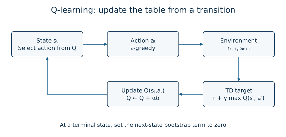
Figure 1 — Q-learning moves the previous value a little toward a target made from the observed reward and the maximum next-state value.
A 5×5 maze has only 25 states and four actions, so 100 table entries are enough. With ε-greedy exploration, experiences gradually propagate the goal value backward through the maze. Setting the learning rate to 1 and fully trusting a single experience leaves it vulnerable to environmental noise, so a value between 0 and 1 is normally used to average across experiences.
2. Off-policy learning and ε-greedy exploration
The target \max_{a'}Q(s',a') is the best estimated action, not necessarily the action that the exploring behavior policy actually took. Q-learning can therefore learn a greedy policy while ε-greedy gathers data. Start with a large ε to cover the state space and decay it slowly. On a physical machine, randomize only within validated candidate commands and keep collision monitoring at the highest priority.
3. Why the table fails for images and continuous values
If a state is every pixel of a camera image and each motor has 256 speed levels, the table cannot fit in practical memory. Nearly identical images would also be treated as unrelated states. DQN approximates the table with a neural network Q_\theta(s,a).
The network maps an image to one Q value per discrete action. For up/down/left/right, the output is (Q(s,\mathrm{up}),Q(s,\mathrm{down}),Q(s,\mathrm{left}),Q(s,\mathrm{right})). The loss is
where D is the replay buffer and \theta^- belongs to the target network. For a terminal transition, y=r.
4. Experience replay: shuffle correlated logs
Robot logs are sequential: frames at t and t+1 look almost identical. A mini-batch made of adjacent frames produces a biased gradient. DQN stores (s_t,a_t,r_{t+1},s_{t+1},done) in a replay buffer and samples random mini-batches.
| Buffer design | Benefit | Cost |
|---|---|---|
| Uniform sampling | simple, weakens temporal correlation | rare failures are sampled less |
| Prioritized replay | focuses on large TD errors | needs importance correction and bookkeeping |
| Fixed-size FIFO | follows a changing environment | old rare failures disappear |
| Episode storage | preserves success/failure context | batches can become correlated again |
Do not overwrite the audit trail with learning preprocessing. Store raw sensor timestamps, requested and actually limited actions, and collision flags separately from normalized training tensors.
5. Target networks: delay the teacher
If the same network being updated computes both target y and prediction Q_\theta simultaneously, the target moves every time. An update meant to shrink the error also moves the next target, leading to divergence or oscillation. DQN keeps a copy Q_{\theta^-} and synchronizes it as \theta^-\leftarrow\theta every few hundred or thousand updates.
Lengthening the sync interval stabilizes the target but makes it stale. Polyak averaging is a smoother alternative:
Record the choice, synchronization interval, loss, and Q-value distribution in the experiment configuration and logs.
6. Overestimation and Double DQN
Taking a maximum over noisy estimates favors an action that happens to look high. Double DQN separates action selection and action evaluation:
This does not remove all bias, but it often reduces unstable Q growth. A missing terminal flag, an incorrect action mask, or an inconsistent reward scale can look similar, so inspect data before changing algorithms.
7. Where DQN belongs in a robot
DQN assumes a finite action set. Discretizing steering angle or joint torque can work for a coarse demonstration, but fine grids grow quickly and create jerky commands. DDPG, TD3, and SAC output continuous actions directly and are often a better fit for torque or hydraulic-valve control.
DQN remains useful for high-level choices: left or right lane, grasp candidate A/B/C, or low/medium/high speed mode. Hand the resulting reference to a PID or MPC layer. The PID article and MPC article show how to keep limits and watchdogs in that lower layer.
8. Draw curves other than reward
Log success rate, collision rate, episode length, mean and maximum Q, TD error, and action frequencies alongside the average episode reward. A rising reward with a rising collision rate usually indicates a reward or termination bug. An exploding Q value with a falling loss suggests a scale mismatch, missing terminal flag, or an incorrect bootstrap target.
Keep evaluation environments separate from training. Change lighting, floor friction, payload, obstacle layout, and communication delay. A policy that succeeds in a simulator but ignores camera exposure, motor dead zones, or battery sag has not demonstrated DQN performance on hardware.
Implementation checklist
- Store state, discrete action, reward, terminal flag, and timestamp as one transition.
- Fix and record ε, learning rate, discount, buffer size, batch size, and target interval.
- Track Q values, TD errors, loss, success/collision rates, and action frequencies by experiment ID.
- Keep replay preprocessing separate from the raw audit log.
- Unit-test action masks, terminal states, timeouts, and invalid sensor values.
- Verify that limits, watchdogs, and emergency stops remain above DQN and work through a network dropout.
- Hold out unseen conditions and failures from training.
Summary
Q-learning turns the Bellman optimality equation into a table update without requiring a known dynamics model. DQN approximates that table with a network, but experience replay and a target network are essential to keep the self-referential target from amplifying noise. DQN is a useful discrete decision layer; continuous torque and safety belong to other controllers. Tracking TD errors, collisions, delays, and Q distributions—not only reward—turns a research script into an auditable robot system.
Does a large Q-value guarantee a large realized reward?
Q is an estimate of expected return. Unfamiliar states or actions can produce large estimation errors.
References
Current step · 2 / 8 · Reinforcement Learning Primer
Comments
Please log in to post a comment
No comments yet.