Contents — find the section you need
Background and reading guide
Background Basic functions, probability and vectors.
Fundamentals · Explanations of principles, structure and trade-offs.
Before a robot can "pick up the cup on the table" or "avoid the pedestrian ahead," it first has to understand, from a camera image, what is there and where. That understanding is the job of Object Detection and Semantic Segmentation. The two are often mentioned in the same breath, but they differ fundamentally — both in how fine-grained their output is and in how the underlying problem is even framed. This article builds both up from the ground, through their 3D counterparts and a clear head-to-head comparison.
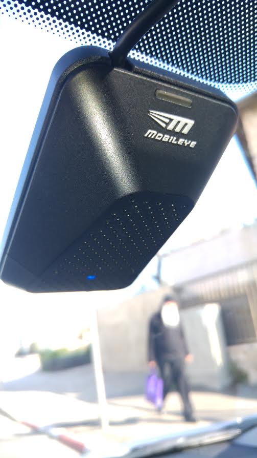 Vehicle perception camera
Image: Car window camera of Mobileye system (Ranbar, CC BY-SA 4.0), Wikimedia Commons. A representative input camera, not a claim about the latest product specifications.

0. What This Article Covers
- What Object Detection and Semantic Segmentation each actually output
- The pipeline Detection runs on (feature extraction → detection head)
- The lineage of landmark algorithms from R-CNN through YOLO, DETR, and DINO, and how their design philosophies differ
- The Two-stage vs. One-stage trade-off, and where Transformer-based detectors fit
- How Segmentation algorithms evolved from FCN to Mask2Former
- A single table that makes the differences between Detection, Semantic, Instance, and Panoptic Segmentation click
- The basics of 3D Object Detection and 3D Semantic Segmentation on point clouds
- How to pick the right technology for robotics, autonomous driving, surveillance, and AR
1. The Short Answer: What Detection and Segmentation Are
In one sentence: Object Detection answers "where in the image is what" with a rectangle (a bounding box), while Semantic Segmentation answers "what is each pixel" by coloring the image in. Both share the same underlying goal — understanding an image — but they answer at completely different resolutions.
Two further tasks build on this pair. Instance Segmentation colors pixels in like Semantic Segmentation, but also distinguishes individual objects of the same class (say, three separate people in a frame). Panoptic Segmentation unifies that Instance Segmentation with the Semantic Segmentation needed for "uncountable" background stuff like road or sky, into a single, maximally complete output. Section 9 below lays out how these four relate in a table.
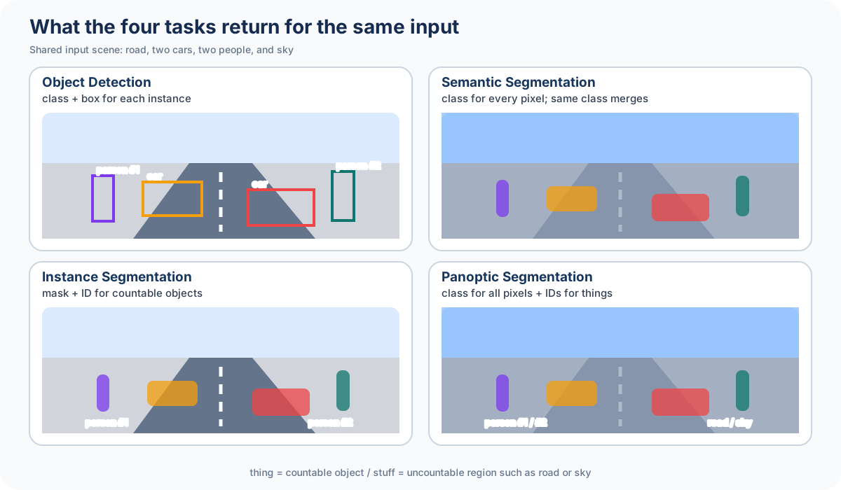
Figure: Duskcoil. Generated from one schematic scene and shared geometry; not measured model output.
2. What Is Object Detection? (Class / Bounding Box / Confidence)
For a single image, Object Detection outputs a set of triples, one per object:
- Class: what the object is (one of a predefined set of categories — "person," "car," "chair," and so on)
- Bounding Box: the rectangle enclosing the object, usually given as a center point plus width and height (x, y, w, h), or as top-left/bottom-right corners (x_1, y_1, x_2, y_2)
- Confidence: a score (0–1) for how sure the model is about that particular box-class pairing
Image Classification returns a single answer — "what is this picture of" — but Object Detection has to answer "how many objects, where, and what kind" all at once. That "the count itself is unknown" property is what makes Detection fundamentally harder than classification. A given image might contain zero objects, or a hundred — the very fact that the number of outputs is variable is the design constraint that drives essentially every trick discussed below.
3. How Is Detection Actually Done?
Facing that variable-output-count problem, essentially every modern Detection algorithm follows the same two-stage pipeline: extract a feature map from the whole image, tile that feature map with a large number of candidate locations (anchor boxes, or the Transformer "queries" discussed later), and for each candidate decide "object or background," and if object, "which class, and what's the precise location."
Figure 2 — The feature extractor (backbone) compresses the image into a feature map, and the detection head performs classification and box regression on top of it simultaneously.
Inside the detection head, two regression/classification problems are effectively solved at once: "is there an object at this candidate location, and if so, which class," and "how much should this candidate (anchor) be shifted to align with the actual object." Combining these into one weighted-sum loss is the multi-task loss used widely from Fast R-CNN onward.
Here p is the predicted class probability, p^{*} the ground-truth class, t the predicted box correction, and t^{*} the target correction derived from the ground-truth box. The indicator \mathbb{1}[p^{*} > 0] means "only compute the location regression error for candidates that actually contain an object, not background" — a background candidate has no ground-truth box to regress toward, so this restriction is natural. \lambda tunes how much weight to give the regression term relative to classification.
4. Landmark Detection Algorithms
The lineage of Detection algorithms is easiest to follow along two axes: "how are candidate regions narrowed down" and "how is the box itself predicted."
R-CNN (Girshick et al., 2014) cut around 2,000 candidate regions out of an image using the classical image-processing algorithm Selective Search, then ran each one through a CNN individually for classification. Accurate, but painfully slow, since the CNN had to run once per candidate region.
Fast R-CNN (Girshick, 2015) ran the whole image through a CNN just once to build a single feature map, then cropped candidate regions out of that feature map (RoI Pooling) — eliminating the redundant per-region computation.
Faster R-CNN (Ren, He, Girshick, Sun, 2015) went one step further and replaced candidate-region generation itself with a small Region Proposal Network (RPN), folding proposal generation, classification, and regression into a single network. These three generations together form the lineage of what's called the Two-stage detector.
SSD (Liu et al., 2016) and YOLO (Redmon et al., 2015–2016) pioneered One-stage detectors, dropping the candidate-region stage entirely and predicting class and box directly from each location on the feature map. Speed jumped dramatically, though early YOLO lagged Two-stage detectors on small-object accuracy.
RetinaNet (Lin et al., 2017) tackled the class-imbalance problem plaguing One-stage detectors — background candidates vastly outnumber object candidates, and training gets dominated by them — with a new loss function, Focal Loss, showing that One-stage detectors could match Two-stage accuracy after all.
FCOS (Tian et al., 2019) went anchor-free altogether: instead of pre-defining a set of anchor boxes at various sizes and aspect ratios, it regresses the distance from each feature-map pixel directly to the object's boundary, sidestepping the hyperparameter tuning that anchor design demands.
DETR, Deformable DETR, and DINO reframe detection with Transformers as a set-prediction problem — the subject of the next section.
5. Two-stage vs. One-stage
Two-stage and One-stage detectors split on exactly one question: does candidate-region narrowing exist as its own independent stage?
| Aspect | Two-stage (e.g. Faster R-CNN) | One-stage (e.g. YOLO) |
|---|---|---|
| Flow | Proposal generation (RPN) → per-region classify & regress | Classify & regress directly at every location on the feature map |
| Accuracy | Generally high, especially on small/dense objects | Recent generations close most of the gap |
| Inference speed | Relatively slow (per-candidate work remains) | Fast, suited to real time |
| Compute cost | Scales with the number of candidates | Roughly proportional to image size, predictable |
| Implementation/tuning difficulty | More stages, more complex | Simpler pipeline |
| Where it fits | Offline processing, accuracy-first inspection/analysis | Real-time perception in vehicles and robots |
Both families long relied on Non-Maximum Suppression (NMS) as post-processing to thin out overlapping candidates. Among the several candidate boxes produced for one object, any whose overlap (IoU: Intersection over Union) with another exceeds a threshold gets discarded, per this definition:
A and B are the regions two boxes occupy; dividing their overlap area by their union area yields a score between 0 and 1. A high IoU signals the two boxes likely point at the same object, so the lower-confidence one gets dropped. NMS works, but it can misfire on densely packed objects — a weakness the DETR family, discussed next, designs away entirely.
6. Detection in the Transformer Era (DETR / Deformable DETR / DINO)
DETR (Carion et al., 2020, Facebook AI) changed how detection is formulated at its core. With no anchors and no NMS, it runs image features through a Transformer encoder and passes a fixed number of "queries" (learnable vectors standing in for candidate objects) through a decoder, directly outputting exactly that many box-class pairs. During training, the predicted set and the ground-truth set are matched one-to-one via the Hungarian algorithm, and the loss is computed against that matching.
y_i is the i-th ground-truth object, \hat{y}_{\sigma(i)} the prediction assigned to it under permutation \sigma, and \mathfrak{S}_N the set of all permutations of N elements. This says: find the permutation \hat{\sigma} that assigns predictions to ground truths one-to-one at minimum total cost — only once that assignment is settled can the usual classification and regression losses be computed. Because no object can ever be assigned more than one prediction, NMS becomes unnecessary by construction.
DETR did have a downside: full self-attention over the whole image is expensive, and the model needed an enormous number of training epochs to converge. Deformable DETR (Zhu et al., 2020) introduced a deformable attention mechanism where each query attends to only a small, learned set of sampling points rather than the entire image, cutting compute while sharply speeding up convergence. DINO (Zhang et al., 2022; "DETR with Improved DeNoising Anchor Boxes") added tricks like contrastive denoising queries for training stability and mixed query selection to seed query initialization from the feature map, reaching the best accuracy among DETR-family detectors at the time. Transformer-based detectors now stand alongside the YOLO family as one of two mainstream directions in production use.
7. What Is Semantic Segmentation?
Semantic Segmentation predicts, for every pixel in an image, which class it belongs to. Its output isn't a bounding box — it's a "class map" at the same resolution as the input image, where every pixel carries a class ID.
Where Object Detection approximates an object with a coarse rectangle, Semantic Segmentation can represent the object's actual outline at pixel resolution — a real strength for thin, elongated shapes like a curb, or intricate outlines like tree branches. The trade-off: even when several instances of the same class appear in a frame, Semantic Segmentation doesn't distinguish them — all "person" pixels get painted the same color, and the count of individuals is lost. Closing that gap is exactly what Instance Segmentation is for, covered below.
8. Landmark Segmentation Algorithms
FCN (Fully Convolutional Network; Long, Shelhamer, Darrell, 2015) stripped the fully-connected layers out of an image-classification CNN, leaving only convolutional layers, so the network could produce pixel-wise predictions directly for input of any size. It's the field's starting point — the first design to establish Semantic Segmentation as a single, end-to-end trainable network.
U-Net (Ronneberger et al., 2015), proposed for medical image segmentation, arranges an encoder (downsampling while extracting features) symmetrically against a decoder (upsampling while reconstructing), and connects matching-resolution encoder and decoder layers directly via "skip connections." That design — preserving fine boundary detail while still producing high-resolution output — became a standard architecture that spread far beyond medicine.
SegNet (Badrinarayanan et al.) remembers, during encoder pooling, exactly which position held the max value ("pooling indices"), then reuses that record during decoder upsampling, restoring boundaries memory-efficiently. PSPNet (Zhao et al., 2017) introduced a Pyramid Pooling Module that averages features over regions at multiple scales, capturing whole-image context that a narrow receptive field alone would miss.
The DeepLab series (Chen et al.) built its core around dilated (atrous) convolution — spreading out the gaps between kernel taps to widen the receptive field without sacrificing resolution — evolving from v1 through v3+ (2018). HRNet (Wang et al., 2019) inverted the usual approach: rather than downsampling and then restoring resolution, it keeps a high-resolution feature stream alive in parallel throughout the entire network, continually exchanging information across resolutions.
SegFormer (Xie et al., 2021) paired a hierarchical Transformer encoder with a lightweight MLP-only decoder, achieving high accuracy and efficiency with a strikingly simple design. Mask2Former (Cheng et al., 2022) reformulated segmentation as "a fixed number of queries, each predicting one mask and one class," restricting each query's attention to the mask region predicted in the previous layer via "masked attention" — delivering both fast convergence and a single architecture that handles Semantic, Instance, and Panoptic segmentation alike.
9. Comparing Detection / Semantic / Instance / Panoptic
The four tasks introduced so far become clear once you organize them along two axes: does it distinguish individual instances of the same class, and does it handle "background" — uncountable stuff like road, sky, or wall.
| Task | Output unit | Distinguishes instances | Handles background | Landmark algorithms | Key metric |
|---|---|---|---|---|---|
| Object Detection | Bounding box | Yes (one box per instance) | No | Faster R-CNN, YOLO, DETR | mAP |
| Semantic Segmentation | Per-pixel class label | No (same class merges into one color) | Yes | FCN, DeepLab, SegFormer | mIoU |
| Instance Segmentation | Per-pixel mask | Yes (separate mask per instance) | No | Mask R-CNN, Mask2Former | AP (mask-IoU based) |
| Panoptic Segmentation | Per-pixel class + instance ID | Yes (foreground only) | Yes (class only, no instance ID) | Panoptic FPN, Mask2Former | PQ (Panoptic Quality) |
As the table makes clear, Panoptic Segmentation (proposed by Kirillov et al., 2019) is the "best of both" of Instance and Semantic Segmentation. Foreground objects — countable things like people and cars — are distinguished per instance, as in Instance Segmentation; background — uncountable things like road and sky — gets only a class label, as in Semantic Segmentation. If you push toward fully and exhaustively describing a single image, you end up exactly at this Panoptic form — a useful way to see how all four tasks relate.
The evaluation metric mIoU (mean Intersection over Union) computes, for each class c, the IoU between the ground-truth region G_c and predicted region P_c, then averages across all classes.
Where Detection's mAP scores agreement at the level of boxes, mIoU scores agreement at the level of pixels — that difference in metric mirrors exactly the difference in what each task treats as "correct."
10. 3D Object Detection
Autonomous vehicles and robots often need to detect an object's 3D position, size, and orientation directly from LiDAR point clouds, not just from 2D images. A point cloud doesn't have the grid structure a 2D image does, so a CNN can't consume it as-is — how to turn this irregular data into something regular is the central design challenge in 3D Object Detection.
SECOND (Yan et al., 2018) divides a point cloud into 3D voxels (cubic cells) and uses sparse convolution to skip the large fraction of voxels that contain no points, sharply cutting the compute cost of 3D CNNs. PointPillars (Lang et al., 2019) simplified this further, aggregating points into vertical "pillars" instead of voxels so the network can process them with ordinary 2D convolution rather than 3D, pushing speed up significantly.
PV-RCNN (Shi et al., 2020) combined the efficiency of voxel-based processing with the precise localization that comes from processing points directly (PointNet-style), in a hybrid Point-Voxel design. CenterPoint (Yin et al., 2021) brought an anchor-free approach to 3D detection: detect an object as a single center point, then regress width, height, depth, and orientation from there, pairing it with PointPillars- or VoxelNet-style backbones for strong accuracy.
Many of these methods share one further design idea: projecting point-cloud information down into a Bird's-Eye View (BEV) — a 2D feature map seen from directly above — before running the detection head. Compressing away height information trades off some detail for the ability to handle "where on the road surface is this object" — the relationship that matters most for driving — within the same framework as an ordinary 2D detector.
11. 3D Semantic Segmentation
3D Semantic Segmentation assigns a class label to every point in a point cloud (or every laser return from a LiDAR). Once again, how to handle irregular point-cloud data is what separates the major approaches.
PointNet++ (Qi et al., 2017) feeds points into the network as-is, with no voxelization or other conversion, grouping neighboring points and aggregating features hierarchically — establishing the foundation for point-based methods. RandLA-Net (Hu et al., 2020) tackled the neighbor-search bottleneck that made large-scale point clouds expensive, combining random sampling with a local feature-aggregation module that compensates for the information random sampling would otherwise lose, reaching practical speeds even on city-scale point clouds.
RangeNet++ (Milioto et al., 2019) skips 3D processing altogether: it projects the point cloud, using the LiDAR's own scan ordering, into a 2D "range image," runs an ordinary 2D CNN over that, and projects the result back into 3D — leveraging the maturity of 2D CNN tooling for speed. Cylinder3D (Zhu et al., 2021) noticed that outdoor LiDAR point clouds radiate outward from the sensor, and voxelized in cylindrical rather than Cartesian coordinates to handle the resulting density falloff at range. SPVNAS (Tang et al., 2020) fused point-based and voxel-based processing via Sparse Point-Voxel convolution, then applied neural architecture search (NAS) to automatically find configurations with a strong accuracy/speed trade-off.
As in the 2D case, 3D Semantic Segmentation's history can be read as a back-and-forth between "keep points as points" (point-based) and "convert to a regular grid" (voxel- or range-image-based), each trading off accuracy, speed, and memory differently.
12. Choosing the Right Approach in Practice
Which of Detection or Segmentation to use, and which specific algorithm, depends heavily on the use case.
- Robotic arms / picking: knowing the exact outline of the target to grasp matters, so Instance Segmentation (e.g. Mask2Former) fits best — a bounding box alone doesn't reveal the object's true shape or a good grasp point.
- Autonomous driving: real-time performance is non-negotiable, so 2D leans on One-stage detectors (the YOLO family), and 3D leans on efficiency-focused BEV-based 3D detectors like PointPillars or CenterPoint. Semantic/Panoptic Segmentation is often layered on top to understand drivable area.
- Surveillance / security cameras: the set of target classes (people, vehicles) is usually limited, and missing a detection matters more than raw speed, opening the door to Two-stage detectors or high-accuracy Transformer-based ones.
- AR/VR: deciding where in the real world to anchor a virtual object typically means using Semantic Segmentation to identify planes and object regions, then applying Sensor Fusion (see the companion article) for true 3D alignment.
On resource-constrained edge devices, speed and footprint usually win out over accuracy — lightweight YOLO variants or a slimmed-down SegFormer. For precise offline analysis (medical imaging, satellite imagery), accuracy comes first, favoring Two-stage detectors or Mask2Former-class models. In practice, that trade-off between real-time performance and accuracy is the single biggest factor in the decision.
For the latest developments — NMS-free architectures, open-vocabulary detection, foundation models in the Segment Anything family — see Technology Trends in Object Detection and Technology Trends in Semantic Segmentation.
13. Summary
Object Detection captures objects as rectangles; Semantic Segmentation captures them pixel by pixel — two image-understanding tasks operating at different resolutions. Detection's lineage runs from Two-stage (Faster R-CNN) through One-stage (YOLO) to Transformer-based detectors that drop anchors and NMS altogether (DETR/DINO); Segmentation's runs from FCN through U-Net and DeepLab to the Transformer-based SegFormer/Mask2Former. On top of that foundation sit Instance Segmentation, which adds per-object distinction, Panoptic Segmentation, which unifies both, and their 3D, point-cloud-based counterparts — and which one to reach for always comes down to whether the moment calls for accuracy or for speed.
What outputs distinguish detection from segmentation?
Detection typically returns boxes and classes; segmentation returns pixel regions. Choose according to localization, contours, and instance-identity needs.
References
Current step · 3 / 8 · Machine Learning Primer
Comments
Please log in to post a comment
No comments yet.