Contents — find the section you need
Background and reading guide
Background Basic frames, velocity and sensor terminology; use the reading guide for background.
Fundamentals · Explanations of principles, structure and trade-offs.
A robot arm's motors can only rotate the angle of each joint, yet what we actually want, almost always, is something stated in task space: "move the hand to this position and orientation." Kinematics is the mathematics that connects these two worlds — "what the joints are doing" and "what we want the hand to do" — and it forms the foundation of every piece of software that controls a robot arm. This article works systematically through forward kinematics, which finds the hand's pose from joint angles; inverse kinematics, which solves the reverse problem; and the Jacobian, which bridges "velocity" between the two spaces — following the equations the whole way.
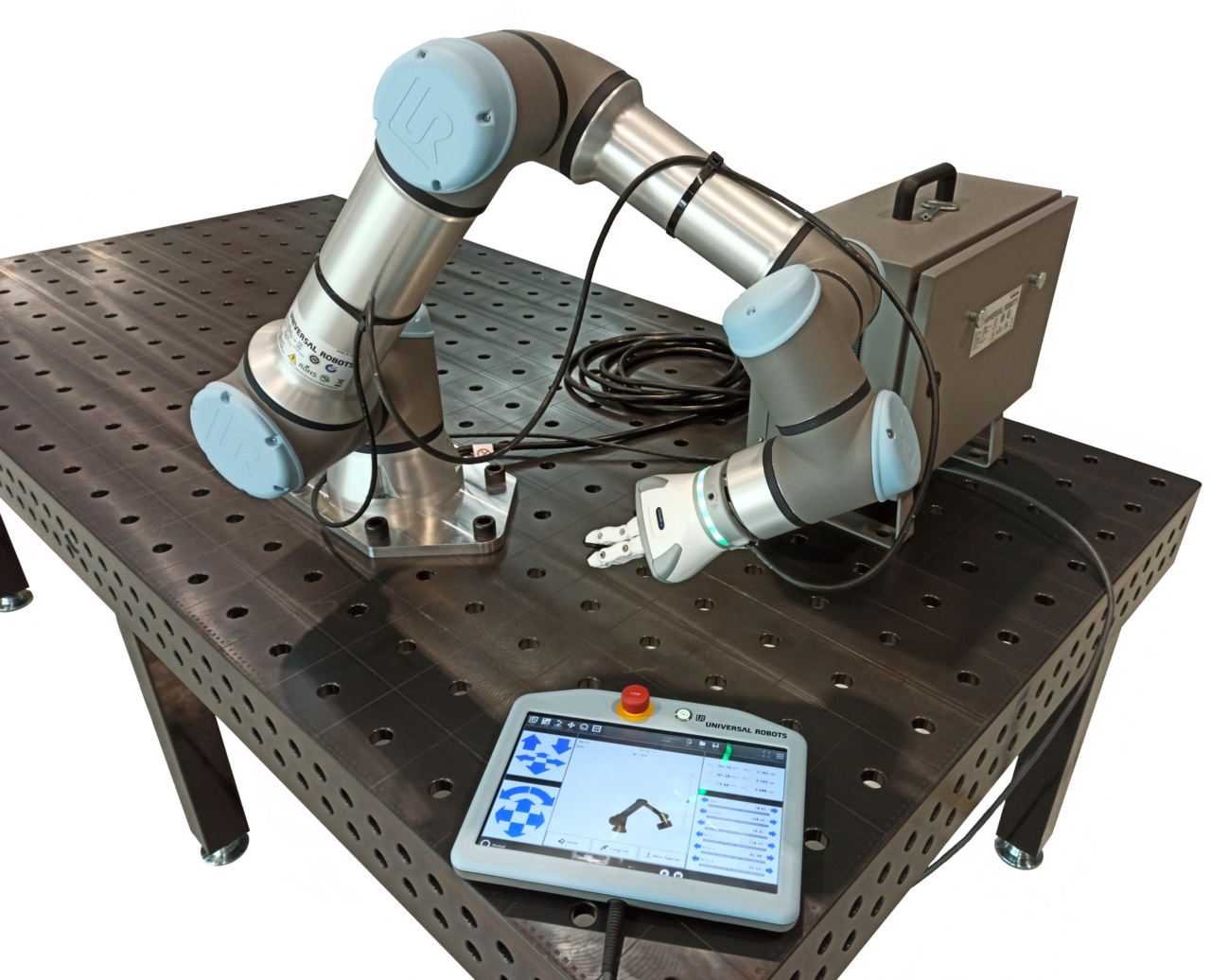 A collaborative robot arm in the field
Image: UR16e robot arm (Auledas, CC BY-SA 4.0), Wikimedia Commons. A representative joint-and-link structure of the kind the article's equations describe, not the kinematic parameters of this specific make or model.

0. What This Article Covers
- What problem robot-arm kinematics solves, and why it's needed
- The relationship between inputs (joint angles, target pose) and outputs (hand pose, joint angles)
- How to build forward kinematics with homogeneous transformation matrices and DH parameters
- Why inverse kinematics is "not necessarily uniquely solvable," and the difference between analytic and numerical methods
- What the Jacobian is, and why it can connect joint velocity to hand velocity
- What happens at a singularity, and why redundant degrees of freedom are useful
- The differences among representative inverse-kinematics algorithms — CCD, FABRIK, Damped Least Squares, and others
- How the use of kinematics differs across industrial robots, humanoids, and CG animation
1. Bottom Line First: What Robot-Arm Kinematics Is
In one sentence: kinematics is the mathematical framework that converts back and forth between two different representations of a robot arm — the angles of its joints (joint space) and the position/orientation of its hand (task space) — using purely geometric relationships, without considering force or motor characteristics.
The phrase "purely geometric relationships" is an important restriction. Kinematics never touches dynamics — how much weight the arm can support, how fast the motors can move. It deals only with the purely geometric questions: "where is the hand when the joint angles are θ?" and "what should the joint angles be to place the hand at this position?" Only once this geometric foundation is in place can we build discussions of force, torque, and trajectory tracking on top of it.
2. Why Is Kinematics Necessary?
A robot arm's motors can only rotate (or extend/retract) each individual joint. But the instructions a human wants to give a robot are, in almost every case, phrased in terms of the hand's (the end effector's) position and orientation — "put this part here," "carry this cup over there." The collection of joint angles (joint space) and the hand's position and pose (task space) look, intuitively, like entirely different quantities: for a 6-axis arm, the joint angles are a set of 6 numbers, while the hand pose is expressed as a 3D position (x, y, z) plus a 3D orientation (rotation) — 6 degrees of freedom in total.
Without a conversion rule linking these two spaces, there's no way to compute "how far to rotate each joint so the hand reaches the target position," and the robot arm simply couldn't perform the motion we intend. Kinematics is the role of stating, as explicit equations, this geometric correspondence between joint space and task space — a correspondence determined by the robot's structure (link lengths, joint layout).
3. What Are the Inputs?
The inputs kinematics deals with depend on which direction we're solving.
- Inputs to Forward Kinematics (FK): a joint vector \boldsymbol{\theta} = (\theta_1, \theta_2, \ldots, \theta_n) collecting each joint's angle (for rotary joints) or slide amount (for prismatic joints). In addition, the robot's structural information (each link's length, each joint axis's layout) is given as a set of constants needed in advance to build the kinematic model.
- Inputs to Inverse Kinematics (IK): the target pose \mathbf{x}_d the hand should achieve. This is a pair of a target position \mathbf{p}_d \in \mathbb{R}^3 and a target orientation (expressed as a rotation matrix or quaternion) R_d; in many cases, especially with numerical methods, the current joint angles \boldsymbol{\theta}_0 are also included as an initial-value input.
The robot's structural information is a "model," not something supplied on every calculation — but if it's inaccurate, both FK and IK will produce results that don't match the real machine. Before working with a robot arm's kinematics at all, this structural model must first be correctly calibrated.
4. What Are We Solving For? What Are the Outputs?
The output of FK is the hand pose \mathbf{x} = (\mathbf{p}, R) given joint angles \boldsymbol{\theta}. This is determined uniquely — once every joint angle is fixed, the link lengths and joint layout are also fixed, so where the hand ends up is geometrically determined as a single answer.
The output of IK is the joint angles \boldsymbol{\theta}^{*} that realize a target pose \mathbf{x}_d. This is where IK differs fundamentally from FK: an IK solution is, in general, not unique. There may be multiple ways to bend the elbow that reach the same hand position (multiple solutions), or the target may simply lie outside the robot's range of motion (outside the reachable workspace), in which case no solution exists at all. This non-uniqueness is precisely what makes IK mathematically harder than FK.
There are also many situations where what we want is not the position or pose itself, but rather the relationship between velocities — "if I move the current joint angles by this much, how much does the hand move?" This is the role of the Jacobian, which we treat in detail in Section 6.
5. Basic Architecture
The processing around kinematics can be organized around the structure of how three transformations — FK, IK, and the Jacobian — connect joint space and task space.
Figure 1 — Forward kinematics (FK) uniquely finds the hand pose from joint angles. Inverse kinematics (IK) solves the reverse direction, but there may be multiple solutions, or none. The Jacobian connects the "velocities" of both spaces through a linear relationship.
The top row represents FK, the middle row IK, and the bottom row the velocity relationship via the Jacobian. FK can always be computed uniquely (left to right), whereas IK (right to left) is a geometric inverse problem that generally requires multiple solution techniques. Because the Jacobian links "rates of change" (velocities) rather than positions or poses themselves, within a linear-algebra framework, it's easier to work with than FK or IK — which is why most numerical IK methods are built on top of it.
6. Representative Algorithms
Homogeneous Transformation Matrices and DH Parameters — Building Forward Kinematics
The basic operation of forward kinematics is to connect the coordinate frames of adjacent links using a homogeneous transformation matrix, which combines rotation and translation.
R_i represents the rotation from link i's coordinate frame to link i-1's coordinate frame, and \mathbf{d}_i represents the translation. For an n-joint arm, the transformation from the base frame to the hand frame is the product of all the individual joint transformations multiplied together.
If these n homogeneous transformation matrices were written from scratch with a different definition for every link, the whole set of equations would have to be rebuilt every time the robot changes. This is why a standardized notation — Denavit-Hartenberg (DH) parameters — is so widely used. Jacques Denavit and Richard Hartenberg proposed this notation in their 1955 paper "A Kinematic Notation for Lower-Pair Mechanisms Based on Matrices," published in the ASME Journal of Applied Mechanics. It expresses the positional relationship between two adjacent joint axes using just four parameters — link length a_i, link twist angle \alpha_i, joint offset d_i, and joint angle \theta_i — allowing each joint's transformation matrix to be assembled in a unified form.
Given this DH parameter table — three constants a_i, \alpha_i, d_i for each joint, plus the variable \theta_i — the forward-kinematics equations for any serial-link robot can be mechanically assembled using the same procedure. This is why industrial-robot manuals and many simulators supply robot specifications in this DH-parameter form.
Analytic IK, Seen Through a 2-Link Planar Arm
Let's look concretely at the idea of analytic IK, which solves the FK equations built from DH parameters in reverse, using the simplest possible example: a 2-link planar arm with link lengths l_1, l_2.
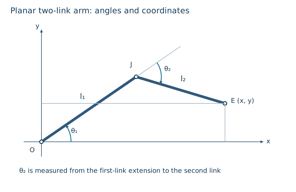
Figure 2 — A 2-link planar arm. The hand E's position (x, y) is determined by the shoulder joint O and elbow joint J angles θ₁, θ₂ and link lengths l₁, l₂ (FK). Conversely, finding θ₁, θ₂ from (x, y) is IK.
Forward kinematics can be written down simply by adding the two link vectors together.
Inverse kinematics finds \theta_1, \theta_2 from a target position (x, y). First, use the law of cosines to find the elbow angle \theta_2.
A solution exists when the right-hand side of this equation falls within [-1, 1], and \theta_2 = \pm\arccos(\cdots) gives two solutions, differing only by sign (bending the elbow up or down). Once \theta_2 is fixed, \theta_1 is determined uniquely (for that choice of \theta_2) from the geometric relationship. This procedure — "derive the inverse trigonometric functions through pure algebraic manipulation" — is analytic IK; it can be written as a closed-form expression for simple mechanisms with 2–3 degrees of freedom, but as the degrees of freedom grow or the joint layout gets more complex, finding a closed-form expression at all generally becomes difficult.
Numerical IK — An Iterative Solution Using the Jacobian
For robots with many degrees of freedom, or mechanisms with no closed-form solution, numerical IK — an iterative computation that gradually approaches the target from the current joint angles — is used instead. This rests on the Jacobian.
Differentiating the hand pose \mathbf{x}(\boldsymbol{\theta}) with respect to the joint angles gives a linear relationship between joint velocity and hand velocity.
J(\boldsymbol{\theta}) is the manipulator Jacobian, an m \times n matrix (m is the task space's degrees of freedom, n the number of joints). The direction in which to update the joint angles to reduce the error \mathbf{e} = \mathbf{x}_d - \mathbf{x}(\boldsymbol{\theta}) from the target pose can be found using the inverse (or pseudoinverse) of the Jacobian.
This idea of an iterative update using the Jacobian pseudoinverse traces back to Daniel E. Whitney's 1969 paper "Resolved Motion Rate Control of Manipulators and Human Prostheses," which proposed a velocity-control framework that included resolving redundant degrees of freedom. However, as the robot approaches a singular configuration (explained in Section 7), J J^{\top} becomes nearly singular (the inverse diverges), and this update becomes unstable. Damped Least Squares (DLS), shown by Charles Wampler in a 1986 paper, suppresses this instability by adding a damping term \lambda^2 I to the inverse computation.
There's a tradeoff: the larger \lambda is, the more numerically stable near singularities, but the slower convergence becomes (the error can only be reduced by a smaller amount each iteration). Because this formula lets you tune convergence speed and stability with a single parameter, \lambda, it's widely adopted in industrial-robot IK solvers for its practicality.
CCD and FABRIK — Iterative Geometric Heuristics
There are also methods that solve IK by repeating more intuitive geometric operations, without using the Jacobian at all. CCD (Cyclic Coordinate Descent) goes joint by joint, from the joint nearest the hand toward the root joint, repeating the simple operation "rotate only this joint to bring the hand as close as possible to the target." It's easy to implement and computationally cheap, but because it moves only one joint at a time, it converges slowly and tends to produce unnatural-looking trajectories.
FABRIK (Forward And Backward Reaching Inverse Kinematics), a method Andreas Aristidou and Joan Lasenby published in Graphical Models in 2011, handles no rotation angles at all — instead it solves IK by repeatedly repositioning each link's joint position as "a point on the straight line to the target, at a distance preserving the link length," moving from hand to root and then from root back to hand. Because it avoids angle computation, it's computationally light and tends to converge to natural-looking poses in few iterations, which is why it's widely used for arm and leg motion in CG animation and video-game characters.
7. How the Algorithms Differ
| Method | Principle | Accuracy | Computational Cost | Robustness Near Singularities | Implementation Difficulty |
|---|---|---|---|---|---|
| DH parameters + homogeneous transforms (FK) | Chains link-by-link transformation matrices | Exact (no error if the model is correct) | Low (matrix products only) | Not applicable (FK has no singularities) | Low |
| Analytic IK | Derives a closed-form solution through trigonometric algebra | Exact (the true solution, if one exists) | Very low | Handled by enumerating solution branches | Low for few DoF, very high as DoF increases |
| Jacobian pseudoinverse | Linearizes the error and updates iteratively | Depends on iteration count; high accuracy once converged | Moderate (repeated matrix operations) | Low (prone to diverging near singularities) | Moderate |
| Damped Least Squares | Adds a damping term to the pseudoinverse | Depends on iteration count and \lambda | Moderate | High (stable even near singularities) | Moderate |
| CCD | Rotates one joint at a time toward the hand target | Depends on iteration count; can fall into local minima | Low | High (no matrix inversion needed) | Low |
| FABRIK | Moves joint positions along a line while preserving link length | Depends on iteration count; tends to converge to visually natural solutions | Low | High | Low |
Analytic IK is "fastest and most accurate when solvable," but as degrees of freedom increase, deriving the equations itself becomes difficult. Numerical methods (Jacobian-based, CCD, FABRIK) can be used generically regardless of degrees of freedom or mechanism, but being iterative, they can't escape the tradeoffs among convergence speed, local minima, and computational cost.
8. Where It Struggles / Difficult Environments
The difficulties inherent to kinematics can be organized broadly into three categories.
Singularities: at certain joint configurations, the rank of the Jacobian J drops, creating a direction in which the hand simply cannot be moved no matter what. For example, with the arm fully extended, there's no combination of joint velocities that can move the hand any further outward. In this state, J J^{\top} approaches a singular matrix, and control laws using the pseudoinverse cause the commanded joint velocities to diverge. The manipulability index w = \sqrt{\det(J J^{\top})}, proposed by Tsuneo Yoshikawa in 1985, is widely used to quantify closeness to a singularity — the closer w is to zero, the closer the configuration is to a singularity.
Multiple solutions and reachability: IK can generally have multiple solutions (different ways of bending the elbow, for instance), and there are also cases where the target pose is physically unreachable given the robot's link lengths and range-of-motion constraints. Unless a numerical method explicitly designs a stopping condition for this "no solution" case, it will keep iterating without ever converging.
Redundant degrees of freedom: for robots with more joints than the task space's degrees of freedom (typically 6) — 7-axis arms, for instance — there are infinitely many combinations of joint angles that achieve the same hand pose. This surplus of degrees of freedom isn't a "troublesome ambiguity" — it's a resource that can be actively used for secondary objectives such as obstacle avoidance, singularity avoidance, or keeping joints near the middle of their range of motion. IK for redundant robots is designed by projecting the gradient of a secondary objective into the Jacobian's null space (the direction of joint velocities that have no effect on the hand pose).
9. Practical Choices
How to implement kinematics depends on the robot's degrees of freedom, application, and real-time requirements.
- Industrial robot arms (welding, assembly, etc., typically 6-axis): with 6 degrees of freedom, many mechanisms admit an analytic IK solution, and in practice, many manufacturers' controllers implement analytic IK directly in firmware. Without needing iterative computation, this is fast and behaves predictably.
- Robot arms with redundant degrees of freedom (7+ axes, collaborative-robot or humanoid arms): analytic solving is either difficult or produces multiple solutions that are cumbersome to handle, so Jacobian-based numerical IK (such as Damped Least Squares) is common. It also makes it easier to design obstacle avoidance and singularity avoidance simultaneously through the null space.
- CG animation, video-game characters, VR/AR avatars: visual naturalness and low computational cost are usually prioritized over physical accuracy, favoring lightweight geometric heuristics such as CCD or FABRIK.
- Mobile manipulators (mobile base + arm) or full-body humanoids: it's necessary to handle not just the arm's own IK but the redundant degrees of freedom of the whole body, including legs and torso, in an integrated way — often using a framework that extends Jacobian-based methods to whole-body kinematics (Whole-Body IK).
In every application, kinematics is never a self-contained technology on its own — a robot arm achieves its intended motion only when combined with the control loop that actually generates joint-velocity and torque commands (LQR Primer, MPC Primer) and the Trajectory Generation Primer, which designs the path the hand should follow along the time axis.
10. Summary (Three-Line Recap)
- Forward kinematics uniquely finds the hand pose from joint angles; inverse kinematics solves the reverse problem, but there may be multiple solutions, or none.
- The Jacobian linearly connects joint velocity to hand velocity, and it's the foundation of numerical IK via the pseudoinverse or Damped Least Squares.
- How you handle the three difficulties of singularities, multiple solutions, and redundant degrees of freedom determines whether analytic or numerical IK is the right choice.
Is there only one joint configuration for an end-effector position?
Multiple solutions or redundancy may exist, and some points are unreachable. Select solutions using joint limits, singularities, and collision constraints.
References
Current step · 14 / 18 · Robotics Primer
Comments
Please log in to post a comment
No comments yet.