Control Engineering Primer: Trajectory Generation — Minimum Jerk, Quintics, and Trapezoidal Profiles

Contents — find the section you need

Background and reading guide

Background Basic functions, calculus and vectors; follow the definitions alongside the equations.

Fundamentals · Explanations of principles, structure and trade-offs.

A path is geometric; a trajectory specifies when that path is traversed and with what velocity, acceleration, and jerk. The center line of an aisle does not tell a loaded cart, a flexible robot arm, or a collaborative manipulator how fast it can turn or stop. A collision-free polyline from a planner can still demand impossible steering, saturate a joint, excite vibration, or spill its payload. Trajectory generation translates geometric feasibility into time- and dynamics-aware executability.

This primer compares trapezoidal/triangular velocity profiles, quintic polynomials, and minimum jerk. It also covers limits, safety, implementation, and the boundary to ROS 2 and path planning. See Path Planning Primer, ROS 2 Primer, and Visual SLAM Primer.

Practical conclusion

Trapezoidal profiles make maximum speed and acceleration clear. Short moves become triangular profiles with no cruise segment. Their ideal acceleration steps imply infinite jerk, which can excite flexible mechanics and payloads.
A quintic polynomial meets position, velocity, and acceleration boundary conditions at both ends. Zero velocity and acceleration endpoints make position through acceleration continuous between segments.
Minimum jerk minimizes $\int j(t)^2dt$ under specified endpoint conditions; with fixed duration it yields a quintic. “Minimum” applies to that selected objective, not automatically to energy, collision risk, or safety.
Monitor position, velocity, acceleration, jerk, limits, current, stopping distance, tracking error, and map freshness together. A trajectory generator is not an E-stop or collision safety system.

Time-parameterizing a path

For spatial path $p(s)$ and progress $s\in[0,1]$ over time $t$ , the trajectory is $p(s(t))$ . Here $\dot s$ is progress rate:

\dot p=\frac{dp}{ds}\dot s,\qquad \ddot p=\frac{d^2p}{ds^2}\dot s^2+\frac{dp}{ds}\ddot s

High curvature raises lateral acceleration. A mobile robot approximately obeys $a_{lat}=v^2\kappa$ , where $\kappa$ is curvature, so a lateral limit $a_{lat,max}$ gives $v\le\sqrt{a_{lat,max}/|\kappa|}$ . Raising speed without smoothing a corner asks a tracker for impossible steering. For an arm, even a smooth end-effector path can create high joint velocity near a kinematic singularity; hand, vehicle, joint, and actuator constraints must be checked together.

Trapezoidal and triangular velocity

For distance $D$ , maximum speed $v_{max}$ , and acceleration magnitude $a_{max}$ , acceleration time is $t_a=v_{max}/a_{max}$ and the accelerate/decelerate-only distance is $D_{tri}=v_{max}^2/a_{max}$ . The acceleration limit is $a_{max}$ . If $D\ge D_{tri}$ , cruise time is

t_c=\frac{D-D_{tri}}{v_{max}}

If $D<D_{tri}$ , cruise disappears and peak speed is $v_p=\sqrt{Da_{max}}$ . This profile is transparent and easy to deploy in simple drives. Its instantaneous acceleration changes are not physical: an S-curve profile limits jerk $j_{max}$ by ramping acceleration, reducing shock and vibration while generally extending the move.

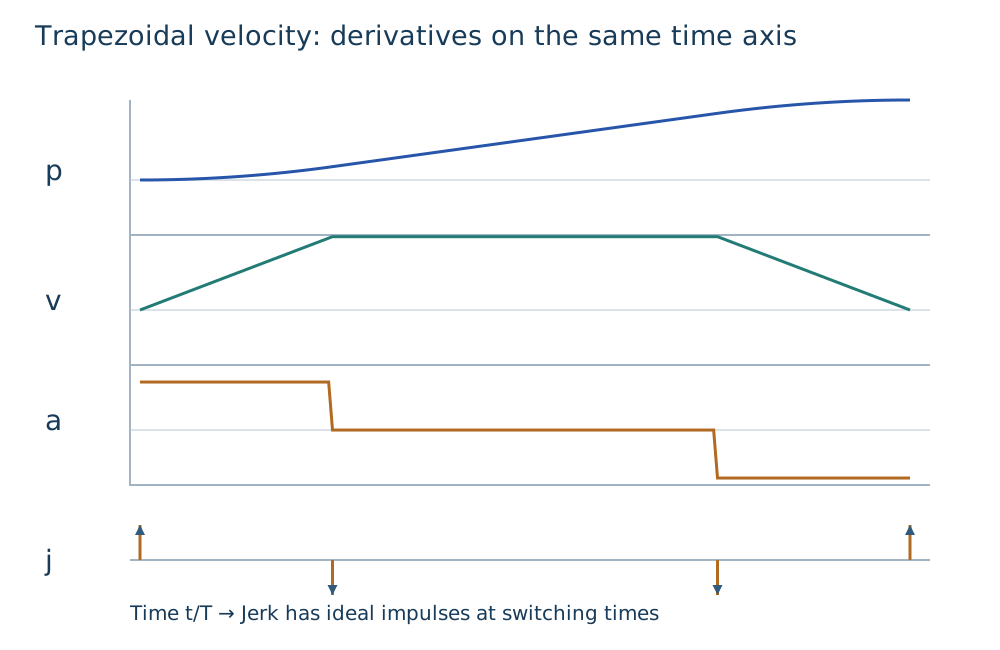
Diagram: Duskcoil, conceptual. In an ideal trapezoid acceleration discontinuities make jerk impulse-like; this is not a measured machine response.

Quintic polynomials and minimum jerk

Let

p(t)=a_0+a_1t+a_2t^2+a_3t^3+a_4t^4+a_5t^5

Six endpoint conditions—position, velocity, acceleration at the initial time and $T$ —determine its six coefficients. In shorthand these are $p(0),\dot p(0),\ddot p(0),p(T),\dot p(T),\ddot p(T)$ and, for a rest-to-rest move, $p(0)=0,p(T)=D,\dot p(0)=\dot p(T)=\ddot p(0)=\ddot p(T)=0$ . For a rest-to-rest move across the selected distance, with $\tau=t/T$ ,

p(t)=D(10\tau^3-15\tau^4+6\tau^5)

Minimum jerk solves

\min_p\int_0^T\left(\frac{d^3p}{dt^3}\right)^2dt

subject to endpoint position, velocity, and acceleration. The Euler–Lagrange condition makes the sixth derivative zero, giving a quintic. Shortening $T$ rapidly increases required velocity, acceleration and jerk, so selecting duration is as consequential as selecting endpoint locations.

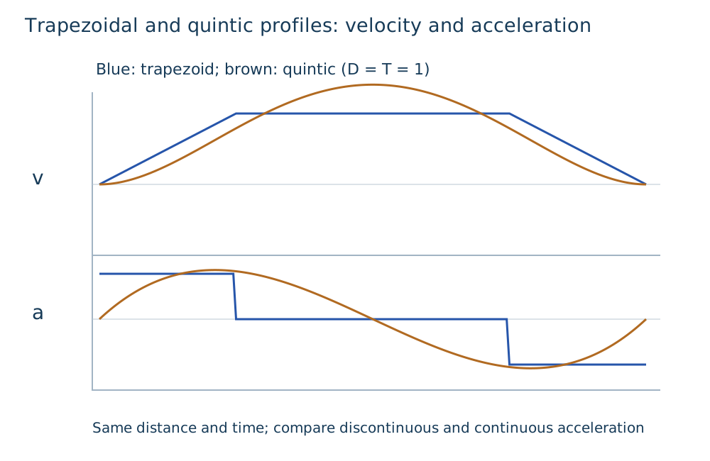
Diagram: Duskcoil. The comparison concerns endpoint smoothness, not a universal measured claim about time, energy, or safety.

Implementation and ROS 2 connection

For one joint, define the move from $q_0$ to $q_f$ , sample $q_d,\dot q_d,\ddot q_d$ from a quintic and supply them to a position/velocity/effort loop; velocity and acceleration can support feedforward. Per-joint interpolation alone may move the end effector near an obstacle, so check Cartesian path, inverse kinematics, joint range, and self-collision too.

For a mobile robot, smooth a route from A* or RRT, apply curvature-dependent speed limits, choose a trapezoid/S-curve/minimum-jerk time law, and translate the generated velocity $v(t)$ to wheel speeds or steering and acceleration. If a person appears in a local costmap, preserving the old smooth arrival is less important than slowing, stopping, or replanning. Global path planning is not local safety.

In ROS 2, distinguish path, trajectory, and control-command timestamps. Define behavior for clock jumps, delayed trajectory messages, cancellation, replacement, and missed control periods; reject stale trajectories and avoid a velocity discontinuity on replacement. ROS 2 lifecycle and hardware boundaries described in ROS 2 Primer help allocate those responsibilities, but do not certify real-time or functional safety.

Limits, safety, and checks

Bounds include $|v|\le v_{max}$ , $|a|\le a_{max}$ and $|j|\le j_{max}$ , but also joint range, torque/current/thermal capacity, tire friction, steering rate, payload, perception, communication latency, and stopping distance. A simple estimate $d_{stop}\simeq v^2/(2a_{brake})+v t_{latency}$ shows that braking distance grows quadratically with speed while sensing and computation delay remain. A generator must be allowed to abandon a trajectory when tracking error, pose uncertainty, saturation, obstacle detection, or stale map exceeds an envelope.

Problem	Likely cause	Monitor	Example response
Error at corners	speed/curvature mismatch	lateral error, steering saturation	slow, smooth route, cap curvature
Payload oscillation	high jerk/flexible mode	IMU, acceleration, vibration	S-curve, longer time, avoid resonance
Jump on goal change	discontinuous boundary velocity	$v,a,j$ , current	bumpless splice and reinterpolation
Cannot stop	delay/braking/map error	freshness, stopping distance	speed limit and safe stop
Joint at limit	IK/time-law mismatch	position, velocity, torque	replan, reject goal, slow

Implementation checklist

Define path versus trajectory, frames, target time, and control period.
Set $v,a,j$ from measured actuator, payload, and stopping limits.
Test triangular/trapezoidal switching and goal replacement boundary conditions.
Check maximum derivatives when reducing quintic duration.
Discard old trajectories on map update, localization jump, tracking deviation, communications loss, or obstacle detection.
Verify independent E-stop, torque limits, and travel limits if trajectory software fails.

Check your understanding

Does a smooth position curve guarantee feasible motion?

Timing determines velocity, acceleration, and jerk. Check their limits as well as the geometric path.

References

Try it in the browser

Lab See how curvature-based speed limits affect trackingRegulated Pure Pursuit Lab — speed through curves and near the goal