Contents — find the section you need
Change parameters and verify
Open the panel, then press Run to load Python. You can stop execution and reset parameters. Results are computed on this device. No Python installation is required.
Local execution steps below are optional for reproducing the source results; they are not required for the browser experiment.
The experiment controls are in English.
Explore timing, mounting position and axes in your browser
Use the panel above to compare ideal examples without ROS or local Python. These calculations explain different sources of disagreement; they do not run a fusion filter, estimate calibration or diagnose a robot. The original diagnostic procedure remains below.
Time offset: Δt is the time of the compared value minus the reference time. The displayed differences are x(t+Δt)−x(t)=vx Δt and heading(t+Δt)−heading(t)=yaw_rate Δt. Positive Δt compares a later value; negative compares an earlier value. At 1 m/s, 90 deg/s and +50 ms, the differences are +0.05 m and +4.5°. These are separate constant-axis translation and constant-angular-rate examples, not an integrated turning trajectory or a prediction of filter error. Time offset is not automatically transport latency or a timestamp-sign convention for a particular driver. Zero motion can hide timing disagreement. No tolerance is recommended.
Mounting position: the lower diagrams describe velocities at one instant. Body axes use x forward, y left, z up; positive yaw is counterclockwise viewed from +z. The supplied base-point velocity is v_base=(vx,0) in body axes. The lever arm r=(rx,ry) points from that base origin to the sensor origin, also in body axes. With ω=yaw_rate × π/180, the mounting-point velocity difference is ω×r=(-ω ry, ω rx) m/s. Thus v_sensor_body=v_base+ω×r. The position plot uses metres; the velocity plot uses m/s with separate scales. Sensor-axis arrows have a display length of 0.15 m. The velocity plot places vectors at a common origin to compare their components, not to depict where the robot travels.
Mounting orientation: R_bs rotates sensor components into body components. The model constructs hypothetical sensor-point linear velocity as v_sensor_components=R_bsᵀ v_sensor_body. Rotating it back gives the velocity of the sensor point, still not the base point. Only after subtracting the known ω×r term does this ideal algebra recover the supplied base velocity. Reuse of the known exact geometry is not a calibration estimate. This is a hypothetical velocity measurement, not raw IMU acceleration or gyro output; acceleration lever-arm effects are not modeled.
The “raw component mismatch” deliberately subtracts sensor-axis numbers from base-axis numbers at another point. It is an example of an invalid comparison, not a filter innovation. Its norm may even cancel to zero for some wrong comparisons. The algebraic recovery residual measures floating-point roundoff after using the same exact model; it is not localization accuracy or evidence that real calibration is correct. The table labels every vector by its point and axes.
Try in-place rotation, zero lever arm, a sensor on the left, reversed rotation and a 90° sensor mounting. Changing mounting yaw changes sensor components but leaves physical body-frame velocity unchanged. Changing Δt affects only the timing exercise. By default the lever arm is 0.2 m and the rate is 90 deg/s, so the lever-arm speed is about 0.314 m/s; the article's separate 1 rad/s example gives 0.2 m/s. Do not confuse degrees/s with radians/s.
All inputs are synthetic and exact. No covariance, noise, observability test, slip, bias, interpolation, TF lookup, clock synchronization, ROS execution or fusion estimator is included. A/B uses matching position and velocity scales; slider limits are teaching choices. For point transforms, use the separate coordinate-transform Lab; for replay conditions, use the replay Lab.
References reviewed 2026-09-20: REP-103 coordinate conventions and Modern Robotics: rigid-body point velocity. The browser uses the site's existing planar rotation helper and the planar form of the rigid-body velocity relation.
Sensör eklemek konumlandırmayı kötüleştiriyorsa, filtre tek şüpheli değildir. Ölçümler, zamanları, kareleri veya birimleri farklıysa doğrudan karşılaştırılamaz. Her bir girişi, ardından füzyona girdiği sınırları kontrol edin.
Teşhis sırasını düzeltin
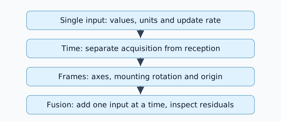
Kısa bir logu yeniden kullanın ve tekerlekleri tek başına, IMU'yu tek başına, ardından her ikisini de inceleyin. Zemin veya sürüş hızını aynı anda değiştirmek nedeni gizler. Sensör füzyonunun temelleri bölümündeki prensipleri gözden geçirin.
Zamanlama hatası hareket hatasına dönüşür
Sabit 1 m/s hızda, 50 ms'lik bir zaman damgası hatası 1\times0.05=0.05 m'lik görünür bir yer değiştirmeye neden olur. 90 derece/s hızda, aynı hata 4,5 derecelik bir dönüş uyumsuzluğuna neden olur. Bunlar sabit hareket hesaplamalarıdır, önerilen toleranslar değildir.
Bir mesaj zaman damgasının sensör alımını mı yoksa sürücü alımını mı gösterdiğini belirleyin. Doğru alım zaman damgalarıyla sabit bir iletim gecikmesi yönetilebilir; ana bilgisayarlar arasında uyuşmayan saatler farklı bir sorundur. Daha uzun bir kuyruk saat sapmasını düzeltmez. Tekrar oynatma sırasında, ilgili tüm düğümlerin aynı simülasyon zamanı yapılandırmasını kullanmasını sağlayın.
Eksenleri ve orijinleri kontrol edin
ROS gövde çerçeveleri normalde x ileri, y sola ve z yukarı kullanır; kamera optik çerçeveleri z ileri, x sağa ve y aşağı kullanır. REP-103'deki kuralları kontrol edin. Bir çerçeveyi yeniden adlandırmak değerlerini döndürmez.
Bir sensör noktasını p_b=R_{bs}p_s+t_{bs} kullanarak dönüştürün. Hem döndürme hem de öteleme önemlidir. Ters öteleme -R^Tt'tür, sadece -t değildir. Kalibrasyonun sensörden gövdeye mi yoksa gövdeden sensöre mi eşlendiğini kaydedin.
Montaj Ofsetleri Hareketi de Değiştirir
Sert bir cisim için, sensördeki hız v_s=v_b+\omega\times r'dır. Dik 0,2 m ofset ve 1 rad/s açısal hız ile hız farkı 0,2 m/s'dir. Dönme merkezinden uzakta bulunan bir sensör, yerinde dönüş sırasında bile hareket eder.
Teşhislerde dönüşleri ve ötelemeyi de dahil edin. Tam dışsal kalibrasyon, yeterince bilgilendirici hareket gerektirir; yalnızca düz sürüş, her serbestlik derecesini tanımlayamayabilir. Çerçeve sorumluluklarını REP-105 ile karşılaştırın.
Kalıntıları ve kovaryansı en son inceleyin
| Belirti | Hipotez | Sonrakini karşılaştırın |
|---|---|---|
| Hata hızla artar | Zamanlama uyumsuzluğu | Farklı hızlarda aynı rota |
| Hata dönüşler sırasında artar | Eksenler, ofset veya zamanlama | Sabit, düz ve sola/sağa dönüşler |
| Giriş eklerken sıçramaları tahmin edin | Çerçeve, birimler veya aşırı güven | Ham girdi ve tahmin kalıntısı |
| Yavaş kayma | Sapma veya kayma | Ham ortalamalar ve gözlemlenebilir yönler |
Kalıntı, gözlem ve tahmin arasındaki farktır. Daha küçük kovaryans güveni artırır; yanlış eksenleri veya zaman damgalarını düzeltmez. Aynı kodlayıcıdan elde edilen konum ve hızı güçlü bir şekilde bağımsız gözlemler olarak ele almak da bilgiyi fazla sayabilir. Resmi robot_localization uygulaması içindeki girdi seçimi ve çerçeve işlemeyi inceleyin.
Her seferinde bir nedeni doğrulayın
Bir ayarı değiştirin, aynı logu karşılaştırın, ardından yeni bir çalıştırma ile doğrulayın. Makul durağan değerler, harekete bağlı senkronizasyon veya montaj hatalarını dışlamaz. SLAM değerlendirmesinden önce, zaman damgası semantiğini, birimleri, TF yayıncılarını ve kalibrasyon yönünü birlikte kaydedin.
Yorumlar
Lütfen önce giriş yapın.
Henüz veri yok.