Contents — find the section you need
Change parameters and verify
Open the panel, then press Run to load Python. You can stop execution and reset parameters. Results are computed on this device. No Python installation is required.
Local execution steps below are optional for reproducing the source results; they are not required for the browser experiment.
The experiment controls are in English.
Explore timing, mounting position and axes in your browser
Use the panel above to compare ideal examples without ROS or local Python. These calculations explain different sources of disagreement; they do not run a fusion filter, estimate calibration or diagnose a robot. The original diagnostic procedure remains below.
Time offset: Δt is the time of the compared value minus the reference time. The displayed differences are x(t+Δt)−x(t)=vx Δt and heading(t+Δt)−heading(t)=yaw_rate Δt. Positive Δt compares a later value; negative compares an earlier value. At 1 m/s, 90 deg/s and +50 ms, the differences are +0.05 m and +4.5°. These are separate constant-axis translation and constant-angular-rate examples, not an integrated turning trajectory or a prediction of filter error. Time offset is not automatically transport latency or a timestamp-sign convention for a particular driver. Zero motion can hide timing disagreement. No tolerance is recommended.
Mounting position: the lower diagrams describe velocities at one instant. Body axes use x forward, y left, z up; positive yaw is counterclockwise viewed from +z. The supplied base-point velocity is v_base=(vx,0) in body axes. The lever arm r=(rx,ry) points from that base origin to the sensor origin, also in body axes. With ω=yaw_rate × π/180, the mounting-point velocity difference is ω×r=(-ω ry, ω rx) m/s. Thus v_sensor_body=v_base+ω×r. The position plot uses metres; the velocity plot uses m/s with separate scales. Sensor-axis arrows have a display length of 0.15 m. The velocity plot places vectors at a common origin to compare their components, not to depict where the robot travels.
Mounting orientation: R_bs rotates sensor components into body components. The model constructs hypothetical sensor-point linear velocity as v_sensor_components=R_bsᵀ v_sensor_body. Rotating it back gives the velocity of the sensor point, still not the base point. Only after subtracting the known ω×r term does this ideal algebra recover the supplied base velocity. Reuse of the known exact geometry is not a calibration estimate. This is a hypothetical velocity measurement, not raw IMU acceleration or gyro output; acceleration lever-arm effects are not modeled.
The “raw component mismatch” deliberately subtracts sensor-axis numbers from base-axis numbers at another point. It is an example of an invalid comparison, not a filter innovation. Its norm may even cancel to zero for some wrong comparisons. The algebraic recovery residual measures floating-point roundoff after using the same exact model; it is not localization accuracy or evidence that real calibration is correct. The table labels every vector by its point and axes.
Try in-place rotation, zero lever arm, a sensor on the left, reversed rotation and a 90° sensor mounting. Changing mounting yaw changes sensor components but leaves physical body-frame velocity unchanged. Changing Δt affects only the timing exercise. By default the lever arm is 0.2 m and the rate is 90 deg/s, so the lever-arm speed is about 0.314 m/s; the article's separate 1 rad/s example gives 0.2 m/s. Do not confuse degrees/s with radians/s.
All inputs are synthetic and exact. No covariance, noise, observability test, slip, bias, interpolation, TF lookup, clock synchronization, ROS execution or fusion estimator is included. A/B uses matching position and velocity scales; slider limits are teaching choices. For point transforms, use the separate coordinate-transform Lab; for replay conditions, use the replay Lab.
References reviewed 2026-09-20: REP-103 coordinate conventions and Modern Robotics: rigid-body point velocity. The browser uses the site's existing planar rotation helper and the planar form of the rigid-body velocity relation.
当添加传感器反而导致定位效果变差时,滤波器并非唯一可能的原因。如果测量值的时间、帧数或单位不同,则无法直接比较。检查每个输入,然后检查其进入融合过程的边界。
修正诊断顺序
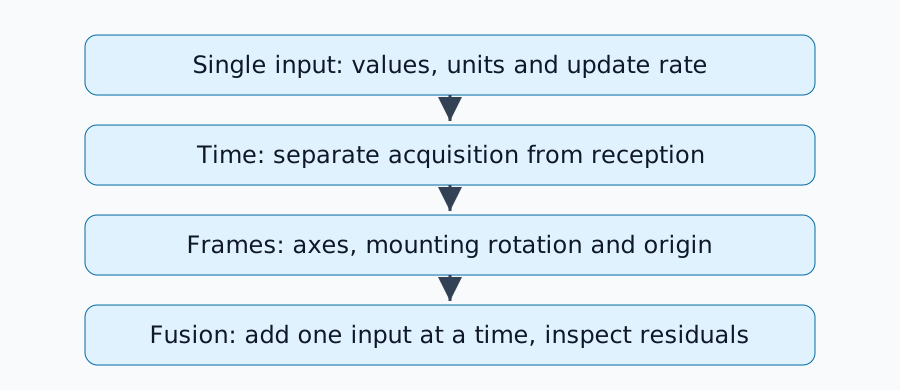
重用一段简短的日志,分别单独检查车轮、IMU,然后再检查两者。同时改变地面或行驶速度会掩盖原因。请复习传感器融合基础中的原理。
时间误差会变成运动误差
在恒定速度 1 m/s 下,50 ms 的时间戳误差会导致 1\times0.05=0.05 m 的表观位移。在 90 度/秒的速度下,同样的误差会导致 4.5 度的旋转偏差。这些是恒定运动情况下的计算结果,并非推荐的公差。
确定消息时间戳表示的是传感器采集还是驱动程序接收。如果采集时间戳正确,固定的传输延迟可能是可以接受的;但主机间时钟不一致则是一个不同的问题。更长的队列并不能纠正时钟偏移。在重放过程中,确保所有相关节点使用相同的仿真时配置。
检查坐标轴和原点
ROS 机体坐标系通常使用 x 轴向前、y 轴向左、z 轴向上;相机光学坐标系使用 z 轴向前、x 轴向右、y 轴向下。请参考 REP-103 中的约定。重命名坐标系不会旋转其值。
使用 p_b=R_{bs}p_s+t_{bs} 变换传感器点。旋转和平移都很重要。逆平移是 -R^Tt,而不是简单的 -t。记录校准是将传感器映射到机体,还是将机体映射到传感器。
安装偏移也会改变运动
对于刚体,传感器处的速度为 v_s=v_b+\omega\times r。垂直偏移 0.2 米,角速度 1 rad/s,速度差为 0.2 米/秒。远离旋转中心的传感器即使在原地转弯时也会移动。
诊断中应包含转弯和平移。完整的外部校准需要足够信息丰富的运动;仅直线行驶可能无法识别所有自由度。将坐标系责任与 REP-105 进行比较。
最后检查残差和协方差
| 症状 | 假设 | 下一步比较 |
|---|---|---|
| 误差随速度增大 | 时序不匹配 | 同一路线不同速度 |
| 转弯时误差增大 | 轴、偏移或时序 | 静止、直线和左右转弯 |
| 估计添加输入时的跳变 | 帧、单位或过度自信 | 原始输入和预测残差 |
| 慢漂移 | 偏差或滑移 | 原始平均值和可观测方向 |
残差是观测值与预测值之间的差异。较小的协方差会增加置信度;但它不会纠正错误的轴或时间戳。将来自同一编码器的位置和速度视为强独立的观测值也可能导致信息过度计数。请检查官方 robot_localization 实现 中的输入选择和帧处理。
一次确认一个原因
更改一个设置,比较相同的日志,然后通过新的运行进行确认。看似合理的稳定值并不能排除运动相关的同步或安装错误。在进行 SLAM 评估 之前,请同时记录时间戳语义、单位、TF 发布者和校准方向。
评论
请先登录。
暂无数据。