Contents — find the section you need
Change parameters and verify
Open the panel, then press Run to load Python. You can stop execution and reset parameters. Results are computed on this device. No Python installation is required.
Local execution steps below are optional for reproducing the source results; they are not required for the browser experiment.
The experiment controls are in English.
Explore timing, mounting position and axes in your browser
Use the panel above to compare ideal examples without ROS or local Python. These calculations explain different sources of disagreement; they do not run a fusion filter, estimate calibration or diagnose a robot. The original diagnostic procedure remains below.
Time offset: Δt is the time of the compared value minus the reference time. The displayed differences are x(t+Δt)−x(t)=vx Δt and heading(t+Δt)−heading(t)=yaw_rate Δt. Positive Δt compares a later value; negative compares an earlier value. At 1 m/s, 90 deg/s and +50 ms, the differences are +0.05 m and +4.5°. These are separate constant-axis translation and constant-angular-rate examples, not an integrated turning trajectory or a prediction of filter error. Time offset is not automatically transport latency or a timestamp-sign convention for a particular driver. Zero motion can hide timing disagreement. No tolerance is recommended.
Mounting position: the lower diagrams describe velocities at one instant. Body axes use x forward, y left, z up; positive yaw is counterclockwise viewed from +z. The supplied base-point velocity is v_base=(vx,0) in body axes. The lever arm r=(rx,ry) points from that base origin to the sensor origin, also in body axes. With ω=yaw_rate × π/180, the mounting-point velocity difference is ω×r=(-ω ry, ω rx) m/s. Thus v_sensor_body=v_base+ω×r. The position plot uses metres; the velocity plot uses m/s with separate scales. Sensor-axis arrows have a display length of 0.15 m. The velocity plot places vectors at a common origin to compare their components, not to depict where the robot travels.
Mounting orientation: R_bs rotates sensor components into body components. The model constructs hypothetical sensor-point linear velocity as v_sensor_components=R_bsᵀ v_sensor_body. Rotating it back gives the velocity of the sensor point, still not the base point. Only after subtracting the known ω×r term does this ideal algebra recover the supplied base velocity. Reuse of the known exact geometry is not a calibration estimate. This is a hypothetical velocity measurement, not raw IMU acceleration or gyro output; acceleration lever-arm effects are not modeled.
The “raw component mismatch” deliberately subtracts sensor-axis numbers from base-axis numbers at another point. It is an example of an invalid comparison, not a filter innovation. Its norm may even cancel to zero for some wrong comparisons. The algebraic recovery residual measures floating-point roundoff after using the same exact model; it is not localization accuracy or evidence that real calibration is correct. The table labels every vector by its point and axes.
Try in-place rotation, zero lever arm, a sensor on the left, reversed rotation and a 90° sensor mounting. Changing mounting yaw changes sensor components but leaves physical body-frame velocity unchanged. Changing Δt affects only the timing exercise. By default the lever arm is 0.2 m and the rate is 90 deg/s, so the lever-arm speed is about 0.314 m/s; the article's separate 1 rad/s example gives 0.2 m/s. Do not confuse degrees/s with radians/s.
All inputs are synthetic and exact. No covariance, noise, observability test, slip, bias, interpolation, TF lookup, clock synchronization, ROS execution or fusion estimator is included. A/B uses matching position and velocity scales; slider limits are teaching choices. For point transforms, use the separate coordinate-transform Lab; for replay conditions, use the replay Lab.
References reviewed 2026-09-20: REP-103 coordinate conventions and Modern Robotics: rigid-body point velocity. The browser uses the site's existing planar rotation helper and the planar form of the rigid-body velocity relation.
जब सेंसर जोड़ने से स्थान निर्धारण में समस्या आती है, तो केवल फ़िल्टर ही संदिग्ध नहीं होता। यदि मापों के समय, फ़्रेम या इकाइयाँ भिन्न हों, तो उनकी सीधी तुलना नहीं की जा सकती। प्रत्येक इनपुट की जाँच करें, फिर उन सीमाओं की जहाँ से यह फ़्यूज़न में प्रवेश करता है।
निदान क्रम को ठीक करें
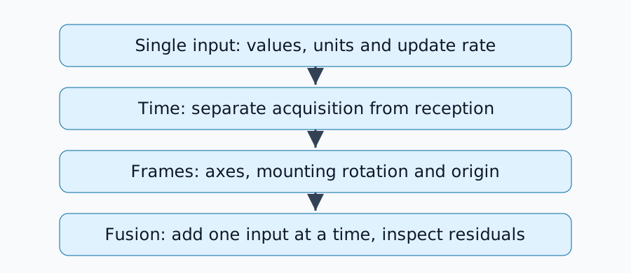
एक छोटा लॉग पुनः उपयोग करें और केवल पहियों की, केवल IMU की, फिर दोनों की जाँच करें। एक ही समय में फ़र्श या ड्राइविंग गति को बदलने से कारण अस्पष्ट हो जाता है। सेंसर फ़्यूज़न के मूल सिद्धांत में दिए गए सिद्धांतों की समीक्षा करें।
समय त्रुटि गति त्रुटि बन जाती है
1 मीटर/सेकंड की स्थिर गति पर, 50 मिलीसेकंड की टाइमस्टैम्प त्रुटि 1\times0.05=0.05 मीटर का आभासी विस्थापन उत्पन्न करती है। 90 डिग्री/सेकंड पर, यही त्रुटि 4.5 डिग्री का घूर्णन बेमेल उत्पन्न करती है। ये स्थिर गति की गणनाएँ हैं, अनुशंसित सहनशीलता नहीं।
यह निर्धारित करें कि संदेश का टाइमस्टैम्प सेंसर अधिग्रहण को दर्शाता है या ड्राइवर द्वारा प्राप्ति को। सही अधिग्रहण टाइमस्टैम्प के साथ एक निश्चित ट्रांसमिशन विलंब को प्रबंधित किया जा सकता है; होस्टों के बीच घड़ियों का असंगत होना एक अलग समस्या है। लंबी कतार घड़ी के अंतर को ठीक नहीं करती है। रीप्ले के दौरान, सुनिश्चित करें कि सभी संबंधित नोड्स एक ही सिमुलेशन-टाइम कॉन्फ़िगरेशन का उपयोग करें।
अक्षों और मूल बिंदुओं की जाँच करें
ROS बॉडी फ़्रेम सामान्यतः x आगे, y बाएँ और z ऊपर का उपयोग करते हैं; कैमरा ऑप्टिकल फ़्रेम z आगे, x दाएँ और y नीचे का उपयोग करते हैं। REP-103 में दिए गए नियमों की जाँच करें। किसी फ़्रेम का नाम बदलने से उसके मानों का घूर्णन नहीं होता है।
p_b=R_{bs}p_s+t_{bs} का उपयोग करके एक सेंसर बिंदु को रूपांतरित करें। घूर्णन और स्थानांतरण दोनों महत्वपूर्ण हैं। व्युत्क्रम स्थानांतरण -R^Tt है, न कि केवल -t। रिकॉर्ड करें कि अंशांकन सेंसर को बॉडी से मैप करता है या बॉडी को सेंसर से।
माउंटिंग ऑफसेट भी गति को प्रभावित करते हैं
एक कठोर पिंड के लिए, सेंसर पर वेग v_s=v_b+\omega\times r है। 0.2 मीटर के लंबवत ऑफसेट और 1 रेडियन/सेकंड के कोणीय वेग के साथ, वेग अंतर 0.2 मीटर/सेकंड है। घूर्णन केंद्र से दूर स्थित सेंसर स्थिर मोड़ के दौरान भी गति करता है।
निदान में स्थानांतरण के साथ-साथ मोड़ों को भी शामिल करें। पूर्ण बाह्य अंशांकन के लिए पर्याप्त जानकारीपूर्ण गति आवश्यक है; केवल सीधी गति से चलने से स्वतंत्रता की प्रत्येक डिग्री की पहचान नहीं हो सकती है। फ्रेम जिम्मेदारियों की तुलना REP-105 से करें।
अवशिष्ट और सहप्रसरण का निरीक्षण अंत में करें
| लक्षण | परिकल्पना | आगे तुलना करें |
|---|---|---|
| गति के साथ त्रुटि बढ़ती है | समय का बेमेल | अलग-अलग गतियों पर एक ही मार्ग |
| मोड़ों के दौरान त्रुटि बढ़ती है | अक्ष, ऑफसेट या समय | स्थिर, सीधी और बाएँ/दाएँ मोड़ |
| इनपुट जोड़ने पर उछाल का अनुमान लगाएं | फ्रेम, इकाइयाँ या अतिविश्वास | कच्चा इनपुट और पूर्वानुमान अवशिष्ट |
धीमा बहाव | पूर्वाग्रह या फिसलन | कच्चे औसत और अवलोकन योग्य दिशाएँ |
अवशिष्ट अवलोकन और पूर्वानुमान के बीच का अंतर है। कम सहप्रसरण से विश्वसनीयता बढ़ती है; यह गलत अक्षों या समय-बिंदुओं को ठीक नहीं करता है। एक ही एनकोडर से प्राप्त स्थिति और वेग को दृढ़ता से स्वतंत्र अवलोकन मानना भी जानकारी की अधिक गणना कर सकता है। आधिकारिक रोबोट_लोकलाइज़ेशन कार्यान्वयन में इनपुट चयन और फ्रेम हैंडलिंग की जाँच करें।
एक समय में एक कारण की पुष्टि करें
एक सेटिंग बदलें, उसी लॉग की तुलना करें, फिर एक नए रन के साथ पुष्टि करें। संभावित स्थिर मान गति-निर्भर सिंक्रनाइज़ेशन या माउंटिंग त्रुटियों को खारिज नहीं करते हैं। SLAM मूल्यांकन से पहले, समय-बिंदु अर्थ, इकाइयाँ, TF प्रकाशक और अंशांकन दिशा को एक साथ रिकॉर्ड करें।
टिप्पणियाँ
पहले लॉग इन करें।
अभी कोई डेटा नहीं है।