Contents — find the section you need
Change parameters and verify
Open the panel, then press Run to load Python. You can stop execution and reset parameters. Results are computed on this device. No Python installation is required.
Local execution steps below are optional for reproducing the source results; they are not required for the browser experiment.
The experiment controls are in English.
Explore timing, mounting position and axes in your browser
Use the panel above to compare ideal examples without ROS or local Python. These calculations explain different sources of disagreement; they do not run a fusion filter, estimate calibration or diagnose a robot. The original diagnostic procedure remains below.
Time offset: Δt is the time of the compared value minus the reference time. The displayed differences are x(t+Δt)−x(t)=vx Δt and heading(t+Δt)−heading(t)=yaw_rate Δt. Positive Δt compares a later value; negative compares an earlier value. At 1 m/s, 90 deg/s and +50 ms, the differences are +0.05 m and +4.5°. These are separate constant-axis translation and constant-angular-rate examples, not an integrated turning trajectory or a prediction of filter error. Time offset is not automatically transport latency or a timestamp-sign convention for a particular driver. Zero motion can hide timing disagreement. No tolerance is recommended.
Mounting position: the lower diagrams describe velocities at one instant. Body axes use x forward, y left, z up; positive yaw is counterclockwise viewed from +z. The supplied base-point velocity is v_base=(vx,0) in body axes. The lever arm r=(rx,ry) points from that base origin to the sensor origin, also in body axes. With ω=yaw_rate × π/180, the mounting-point velocity difference is ω×r=(-ω ry, ω rx) m/s. Thus v_sensor_body=v_base+ω×r. The position plot uses metres; the velocity plot uses m/s with separate scales. Sensor-axis arrows have a display length of 0.15 m. The velocity plot places vectors at a common origin to compare their components, not to depict where the robot travels.
Mounting orientation: R_bs rotates sensor components into body components. The model constructs hypothetical sensor-point linear velocity as v_sensor_components=R_bsᵀ v_sensor_body. Rotating it back gives the velocity of the sensor point, still not the base point. Only after subtracting the known ω×r term does this ideal algebra recover the supplied base velocity. Reuse of the known exact geometry is not a calibration estimate. This is a hypothetical velocity measurement, not raw IMU acceleration or gyro output; acceleration lever-arm effects are not modeled.
The “raw component mismatch” deliberately subtracts sensor-axis numbers from base-axis numbers at another point. It is an example of an invalid comparison, not a filter innovation. Its norm may even cancel to zero for some wrong comparisons. The algebraic recovery residual measures floating-point roundoff after using the same exact model; it is not localization accuracy or evidence that real calibration is correct. The table labels every vector by its point and axes.
Try in-place rotation, zero lever arm, a sensor on the left, reversed rotation and a 90° sensor mounting. Changing mounting yaw changes sensor components but leaves physical body-frame velocity unchanged. Changing Δt affects only the timing exercise. By default the lever arm is 0.2 m and the rate is 90 deg/s, so the lever-arm speed is about 0.314 m/s; the article's separate 1 rad/s example gives 0.2 m/s. Do not confuse degrees/s with radians/s.
All inputs are synthetic and exact. No covariance, noise, observability test, slip, bias, interpolation, TF lookup, clock synchronization, ROS execution or fusion estimator is included. A/B uses matching position and velocity scales; slider limits are teaching choices. For point transforms, use the separate coordinate-transform Lab; for replay conditions, use the replay Lab.
References reviewed 2026-09-20: REP-103 coordinate conventions and Modern Robotics: rigid-body point velocity. The browser uses the site's existing planar rotation helper and the planar form of the rigid-body velocity relation.
센서를 추가할수록 위치 추정 정확도가 떨어지는 경우, 필터만 의심할 수는 없습니다. 측정값의 시간, 프레임 또는 단위가 다르면 직접 비교할 수 없습니다. 각 입력값을 확인한 후, 센서 융합에 들어가는 경계를 점검하십시오.
진단 순서 수정
개별 입력값, 시간, 프레임, 마지막으로 센서 융합 순서로 점검
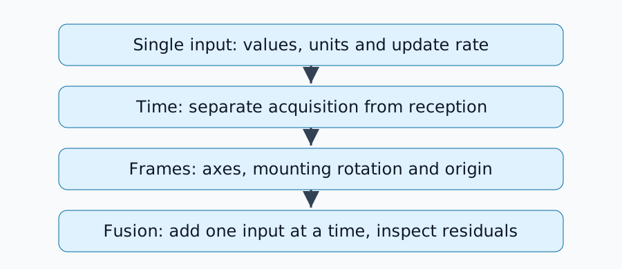
짧은 로그를 재사용하여 바퀴 센서만, IMU 센서만, 그리고 둘 다를 차례로 점검하십시오. 바닥이나 주행 속도를 동시에 변경하면 원인을 파악하기 어려워집니다. 센서 융합 기본 사항의 원리를 다시 검토하십시오.
타이밍 오류가 동작 오류로 이어짐
일정한 속도 1m/s에서 50ms의 타임스탬프 오류는 1\times0.05=0.05m의 겉보기 변위를 발생시킵니다. 90도/s의 속도에서는 동일한 오류가 4.5도의 회전 불일치를 발생시킵니다. 이는 일정한 운동 상태를 가정한 계산이며, 권장되는 허용 오차가 아닙니다.
메시지 타임스탬프가 센서 데이터 획득을 나타내는지, 드라이버 수신을 나타내는지 확인하십시오. 정확한 데이터 획득 타임스탬프가 있다면 고정된 전송 지연은 관리 가능할 수 있지만, 호스트 간 클록 불일치는 별개의 문제입니다. 큐 길이가 길다고 해서 클록 오프셋이 수정되는 것은 아닙니다. 재생 시 모든 관련 노드가 동일한 시뮬레이션 시간 구성을 사용하도록 하십시오.
축 및 원점 확인
ROS 바디 프레임은 일반적으로 x축이 앞쪽, y축이 왼쪽, z축이 위쪽을 사용합니다. 카메라 광학 프레임은 z축이 앞쪽, x축이 오른쪽, y축이 아래쪽을 사용합니다. REP-103의 규칙을 확인하십시오. 프레임 이름을 변경해도 값은 회전하지 않습니다.
p_b=R_{bs}p_s+t_{bs}을 사용하여 센서 포인트를 변환하십시오. 회전과 이동 모두 중요합니다. 역변환은 -R^Tt이며, 단순히 -t이 아닙니다. 보정 시 센서를 바디에 매핑하는지, 바디를 센서에 매핑하는지 기록하십시오.
장착 오프셋 또한 움직임에 영향을 미칩니다.
강체의 경우 센서에서의 속도는 v_s=v_b+\omega\times r입니다. 수직 방향으로 0.2m 오프셋이 있고 각속도가 1rad/s일 때, 속도 차이는 0.2m/s입니다. 회전 중심에서 벗어난 센서는 제자리 회전 중에도 움직입니다.
진단에 병진 운동뿐만 아니라 회전 운동도 포함해야 합니다. 완전한 외부 교정을 위해서는 충분히 유용한 움직임 데이터가 필요합니다. 직선 주행만으로는 모든 자유도를 식별할 수 없을 수 있습니다. 프레임별 책임 범위를 REP-105와 비교하십시오.
잔차 및 공분산은 마지막에 검사합니다.
| 증상 | 가설 | 다음 비교 항목 |
|---|---|---|
| 속도가 증가함에 따라 오차가 증가함 | 타이밍 불일치 | 다른 속도로 동일 경로 주행 |
| 회전 중 오차가 증가함 | 축, 오프셋 또는 타이밍 | 정지, 직선 및 좌/우회전 |
| 입력 추가 시 오차 급증 추정 | 프레임, 단위 또는 과신 | 원시 입력 및 예측 잔차 |
| 느린 드리프트 | 편향 또는 슬립 | 원시 평균 및 관측 가능한 방향 |
잔차는 관측값과 예측값의 차이입니다. 공분산이 작을수록 신뢰도가 높아지지만, 잘못된 축이나 타임스탬프를 수정하지는 않습니다. 동일한 엔코더에서 얻은 위치와 속도를 매우 독립적인 관측값으로 처리하면 정보가 과다하게 계산될 수 있습니다. 공식 로봇 위치 추정 구현의 입력 선택 및 프레임 처리 방식을 검토하십시오.
한 번에 하나의 원인 확인
설정을 하나 변경하고 동일한 로그를 비교한 다음 새 실행으로 확인합니다. 그럴듯한 정지 상태 값이 움직임에 따른 동기화 또는 장착 오류를 배제하는 것은 아닙니다. SLAM 평가 전에 타임스탬프 의미, 단위, TF 게시자 및 보정 방향을 함께 기록하십시오.
댓글
먼저 로그인해 주세요.
아직 데이터가 없습니다.