Contents — find the section you need
Change parameters and verify
Open the panel, then press Run to load Python. You can stop execution and reset parameters. Results are computed on this device. No Python installation is required.
Local execution steps below are optional for reproducing the source results; they are not required for the browser experiment.
The experiment controls are in English.
Explore timing, mounting position and axes in your browser
Use the panel above to compare ideal examples without ROS or local Python. These calculations explain different sources of disagreement; they do not run a fusion filter, estimate calibration or diagnose a robot. The original diagnostic procedure remains below.
Time offset: Δt is the time of the compared value minus the reference time. The displayed differences are x(t+Δt)−x(t)=vx Δt and heading(t+Δt)−heading(t)=yaw_rate Δt. Positive Δt compares a later value; negative compares an earlier value. At 1 m/s, 90 deg/s and +50 ms, the differences are +0.05 m and +4.5°. These are separate constant-axis translation and constant-angular-rate examples, not an integrated turning trajectory or a prediction of filter error. Time offset is not automatically transport latency or a timestamp-sign convention for a particular driver. Zero motion can hide timing disagreement. No tolerance is recommended.
Mounting position: the lower diagrams describe velocities at one instant. Body axes use x forward, y left, z up; positive yaw is counterclockwise viewed from +z. The supplied base-point velocity is v_base=(vx,0) in body axes. The lever arm r=(rx,ry) points from that base origin to the sensor origin, also in body axes. With ω=yaw_rate × π/180, the mounting-point velocity difference is ω×r=(-ω ry, ω rx) m/s. Thus v_sensor_body=v_base+ω×r. The position plot uses metres; the velocity plot uses m/s with separate scales. Sensor-axis arrows have a display length of 0.15 m. The velocity plot places vectors at a common origin to compare their components, not to depict where the robot travels.
Mounting orientation: R_bs rotates sensor components into body components. The model constructs hypothetical sensor-point linear velocity as v_sensor_components=R_bsᵀ v_sensor_body. Rotating it back gives the velocity of the sensor point, still not the base point. Only after subtracting the known ω×r term does this ideal algebra recover the supplied base velocity. Reuse of the known exact geometry is not a calibration estimate. This is a hypothetical velocity measurement, not raw IMU acceleration or gyro output; acceleration lever-arm effects are not modeled.
The “raw component mismatch” deliberately subtracts sensor-axis numbers from base-axis numbers at another point. It is an example of an invalid comparison, not a filter innovation. Its norm may even cancel to zero for some wrong comparisons. The algebraic recovery residual measures floating-point roundoff after using the same exact model; it is not localization accuracy or evidence that real calibration is correct. The table labels every vector by its point and axes.
Try in-place rotation, zero lever arm, a sensor on the left, reversed rotation and a 90° sensor mounting. Changing mounting yaw changes sensor components but leaves physical body-frame velocity unchanged. Changing Δt affects only the timing exercise. By default the lever arm is 0.2 m and the rate is 90 deg/s, so the lever-arm speed is about 0.314 m/s; the article's separate 1 rad/s example gives 0.2 m/s. Do not confuse degrees/s with radians/s.
All inputs are synthetic and exact. No covariance, noise, observability test, slip, bias, interpolation, TF lookup, clock synchronization, ROS execution or fusion estimator is included. A/B uses matching position and velocity scales; slider limits are teaching choices. For point transforms, use the separate coordinate-transform Lab; for replay conditions, use the replay Lab.
References reviewed 2026-09-20: REP-103 coordinate conventions and Modern Robotics: rigid-body point velocity. The browser uses the site's existing planar rotation helper and the planar form of the rigid-body velocity relation.
Ketika penambahan sensor memperburuk lokalisasi, filter bukanlah satu-satunya penyebab masalah. Pengukuran tidak dapat dibandingkan secara langsung jika waktu, frame, atau satuannya berbeda. Periksa setiap input, lalu batas-batas di mana input tersebut masuk ke dalam fusi.
Perbaiki urutan diagnostik
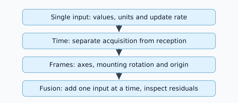
Gunakan kembali log pendek dan periksa roda saja, IMU saja, lalu keduanya. Mengubah lantai atau kecepatan mengemudi secara bersamaan mengaburkan penyebabnya. Tinjau prinsip-prinsip dalam dasar-dasar fusi sensor.
Kesalahan waktu menjadi kesalahan gerak
Pada kecepatan konstan 1 m/s, kesalahan stempel waktu 50 ms menciptakan perpindahan semu 1\times0.05=0.05 m. Pada 90 derajat/s, kesalahan yang sama menciptakan ketidaksesuaian rotasi 4,5 derajat. Ini adalah perhitungan gerak konstan, bukan toleransi yang direkomendasikan.
Tentukan apakah stempel waktu pesan menunjukkan akuisisi sensor atau penerimaan driver. Penundaan transmisi tetap mungkin dapat dikelola dengan stempel waktu akuisisi yang benar; jam yang tidak sesuai antar host adalah masalah yang berbeda. Antrian yang lebih panjang tidak memperbaiki offset jam. Selama pemutaran ulang, pastikan semua node yang relevan menggunakan konfigurasi waktu simulasi yang sama.
Periksa sumbu dan titik asal
Bingkai badan ROS biasanya menggunakan x ke depan, y ke kiri, dan z ke atas; bingkai optik kamera menggunakan z ke depan, x ke kanan, dan y ke bawah. Periksa konvensi di REP-103. Mengganti nama bingkai tidak memutar nilainya.
Transformasikan titik sensor menggunakan p_b=R_{bs}p_s+t_{bs}. Baik rotasi maupun translasi penting. Translasi inversnya adalah -R^Tt, bukan hanya -t. Catat apakah kalibrasi memetakan sensor ke badan atau badan ke sensor.
Offset pemasangan juga mengubah gerakan
Untuk benda kaku, kecepatan pada sensor adalah v_s=v_b+\omega\times r. Dengan offset tegak lurus 0,2 m dan kecepatan sudut 1 rad/s, perbedaan kecepatannya adalah 0,2 m/s. Sensor yang jauh dari pusat rotasi bergerak bahkan selama putaran di tempat.
Sertakan putaran serta translasi dalam diagnostik. Kalibrasi ekstrinsik penuh membutuhkan gerakan yang cukup informatif; mengemudi lurus saja mungkin tidak mengidentifikasi setiap derajat kebebasan. Bandingkan tanggung jawab bingkai dengan REP-105.
Periksa residual dan kovariansi terakhir
| Gejala | Hipotesis | Bandingkan selanjutnya |
|---|---|---|
| Kesalahan meningkat seiring kecepatan | Ketidaksesuaian waktu | Rute yang sama pada kecepatan berbeda |
| Kesalahan meningkat selama belokan | Sumbu, offset, atau waktu | Diam, lurus, dan belokan kiri/kanan |
| Estimasi lompatan saat menambahkan input | Bingkai, satuan, atau kepercayaan diri yang berlebihan | Input mentah dan residual prediksi |
| Pergeseran lambat | Bias atau slip | Rata-rata mentah dan arah yang dapat diamati |
Residual adalah perbedaan antara pengamatan dan prediksi. Kovarians yang lebih kecil meningkatkan kepercayaan; namun tidak mengoreksi sumbu atau stempel waktu yang salah. Memperlakukan posisi dan kecepatan yang diperoleh dari encoder yang sama sebagai pengamatan yang sangat independen juga dapat menghitung informasi secara berlebihan. Periksa pemilihan input dan penanganan frame dalam implementasi_lokalisasi_robot resmi.
Konfirmasikan satu penyebab pada satu waktu
Ubah satu pengaturan, bandingkan log yang sama, lalu konfirmasikan dengan percobaan baru. Nilai stasioner yang masuk akal tidak mengesampingkan sinkronisasi yang bergantung pada gerakan atau kesalahan pemasangan. Sebelum evaluasi SLAM, catat semantik stempel waktu, satuan, penerbit TF, dan arah kalibrasi secara bersamaan.
Komentar
Silakan masuk terlebih dahulu.
Belum ada data.