Contents — find the section you need
Background and reading guide
Background Basic force, motion and energy terminology; use the linked background explanations.
Fundamentals · Explanations of principles, structure and trade-offs.
A LiDAR point cloud can make walls and roads look beautifully precise. A planner needs a different answer: where can the vehicle body fit, what space has never been observed, how uncertain is an obstacle, and when should the trace of a moving pedestrian disappear? An occupancy grid divides continuous space into cells and accumulates the probability that each cell is occupied.
It is not merely a black-and-white image. Cells traversed by a range ray provide free-space evidence; a valid endpoint provides occupied evidence; cells no ray has observed remain unknown. Painting unknown space as free can route a vehicle through an unseen alley or behind a wall. This article connects one range update to Bayesian mapping, SLAM, dynamics, 3D representations, planning, and safety evaluation.
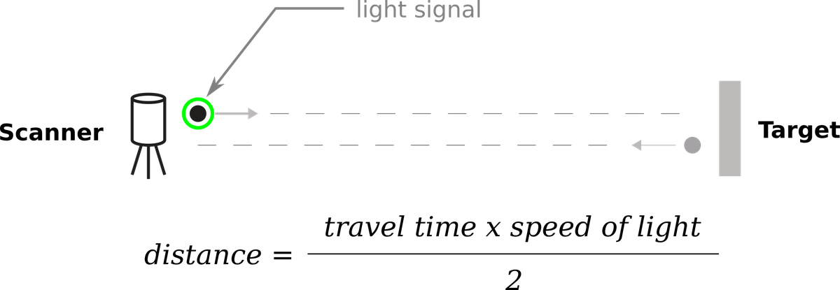 LiDAR as an occupancy-grid observation source
Image: Concept of LiDAR (Cartographer3d, CC BY-SA 4.0), Wikimedia Commons. This is a time-of-flight concept, not a specific vehicle or product implementation of the grid described here.

The short conclusion
- Store a probability for each cell. Values near 0.5 represent unknown, values near one occupied, and values near zero free.
- Log-odds turns recursive Bayesian evidence into addition. Clamp its range so an old, strongly believed obstacle can eventually be cleared.
- Mark a valid return endpoint and ray-trace free space before it. Do not give maximum range, no return, glass, dust, snow, and hardware errors the same inverse model.
- A SLAM map supports localization and persistent structure; a rolling local costmap supports immediate collision avoidance. Separate static and dynamic time scales.
- The vehicle is not a point. Inflate obstacles by footprint, pose and tracking uncertainty, controller error, and stopping margin before planning.
- Semantic occupancy, future occupancy flow, and neural implicit maps are active research directions, but collision-query latency, calibration, and unknown-space behavior remain decisive.
From a range ray to cells
Figure 1 — An inverse sensor model marks the endpoint and clears cells before it. Gray unknown space is not free space.
For origin (x_0,y_0) and resolution r, a world point (x,y) maps to
Halving r roughly quadruples 2D memory and multiplies dense 3D voxel memory by eight. Resolution below sensor and pose uncertainty creates flicker rather than genuine precision.
Transforms among a persistent map frame, continuous odometry frame, vehicle body, and sensor must be evaluated at the measurement timestamp. A current point cloud transformed with an old vehicle pose turns straight walls into slanted bands. Many apparent mapping defects are clock and frame defects.
Bayesian and log-odds update
Let O_i be occupancy of cell m_i, observations through time t be z_{1:t}, and poses be x_{1:t}. The map stores
Classic grids assume cell independence for tractability and use an inverse sensor model P(O_i\mid z_t,x_t). This discards spatial correlation such as continuity of a wall, but permits efficient local updates.
Define log-odds
The recursive update becomes
With p_0=0.5, l_0=0. Occupied evidence adds a positive increment and free evidence a negative increment. Recover probability through
In practice, clamp to l_{min}\le l_{t,i}\le l_{max}. Without saturation, an object observed for hours may require hundreds of free observations to disappear after it moves. Clamping is a decision about how strongly the system can revise history, not only numerical hygiene.
The inverse sensor model
For a 2D scan, Bresenham or DDA enumerates cells along a beam. A valid endpoint marks occupancy and preceding cells receive free evidence. Different return states require different policies:
- A valid return can mark the endpoint and clear before it.
- A maximum-range or no-return sample may clear within a verified range, depending on device semantics.
- Below-minimum-range data should not clear a near-field blind zone.
- Rain, snow, insects, and dust benefit from spatial and temporal consistency filters.
- Glass and low-reflectance surfaces can make no return unsafe evidence of free space.
Camera depth, stereo, and semantic segmentation can be projected to the ground. Monocular class output alone has no accurate range. If projection assumes a road plane, learned depth, or object dimensions, spread the corresponding uncertainty. A sparse feature map used by Visual SLAM and a collision grid have different jobs.
Pose uncertainty and loop closure
Let g(x,z) be the function that transforms sensor point z into world coordinates via pose x; with pose covariance P_x and measurement covariance R_z, first-order propagation of the linearized point gives
Strongly marking one tiny cell while localization is uncertain thickens walls on repeated passes. Distribute evidence spatially or update in submap coordinates. When loop closure changes old poses, points irreversibly burned into one global raster are hard to repair; pose graphs and submaps can be reassembled after optimization. See LiDAR SLAM Primer.
Separate static, local, and dynamic layers
| Layer | Time scale | Examples | Update policy |
|---|---|---|---|
| static | days to years | wall, curb, building | SLAM/HD map, controlled updates |
| temporary | seconds | parked vehicle, dropped object | marking, clearing, decay |
| dynamic | tenths to seconds | vehicle, pedestrian, cyclist | tracking and future occupancy |
| semantic/rules | map version | lane, stop line, keepout | versioned source |
| safety margin | control cycle | footprint, stopping margin | speed- and uncertainty-dependent |
A simple decay is
Too small a \tau erases a stationary obstacle; too large leaves trails behind moving traffic. Track dynamic objects separately where possible and prevent their observations from permanently contaminating static structure.
Future occupancy P(O_{i,k}) or occupancy flow represents where space may be occupied at future step k. Unlike a box detector, it can represent unclassified obstacles and multiple spatial hypotheses. Calibration remains critical: a 0.9 occupancy prediction should be correct about 90% of the time within the evaluated distribution.
2D, elevation, voxels, and BEV
A 2D grid is fast but cannot naturally represent overhangs, branches, the gap under a truck, or slopes. A 2.5D elevation map stores height statistics per cell; a voxel grid discretizes volume; OctoMap compresses occupied volume in an octree.
Automated-driving networks increasingly transform camera, LiDAR, and radar features into bird's-eye view and predict occupancy, semantics, and motion. Learned completion can infer occluded regions, but its probability may be overconfident outside training data. Evaluate reliability diagrams, expected calibration error, distance, weather, geography, and sensor-fault slices.
When reducing 3D to a 2D planning layer, explicitly define the obstacle-height band. A low curb, traversable grass, and an overhead beam cannot share one projection rule.
From occupancy to cost and control
Planning uses collision and proximity cost rather than raw occupancy alone. One inflation model for obstacle distance d is
Account for vehicle footprint and swept volume, pose and tracking covariance, controller tracking error, and stopping distance. A circular robot radius is insufficient for a long vehicle during a turn.
Path Planning Primer explains A and Hybrid A search over costs. MPC Primer optimizes a predicted trajectory subject to vehicle and obstacle constraints. If mapping runs at 5 Hz and control at 50 Hz, the controller must inspect the grid timestamp and bound behavior under stale data.
ROS 2 Nav2 Costmap2D layers static maps, obstacles, voxels, inflation, keepout zones, and speed filters through plugins. Ordering matters: an obstacle inserted after inflation will not receive the expected margin.
Cooperative occupancy over V2X
V2X can share an occluded region before ego sensors see it. The tile needs source frame, measurement time, sender pose covariance, and provenance. If several vehicles relay the same roadside observation, treating them as independent evidence double-counts confidence.
During communication delay \Delta t, a dynamic object moves about v\Delta t. Separate static from dynamic content, propagate motion, and never override local evidence merely because a packet is signed. A compromised sender can mark the entire road blocked; physical consistency and source diversity are required beyond authentication.
Failure patterns and safety response
Treating unknown as free
Initializing unobserved cells as zero routes through space the sensor has never seen. An exploration robot can assign a separate cost to the value of entering unknown space; a road vehicle should treat unknown inside its stopping distance conservatively.
Clearing too aggressively
One “no return” observation can erase a wall when the target is glass or rain has attenuated the signal. Use different update magnitudes for occupied and free evidence, require repeated confirmation, and assign confidence by sensor type.
Using a stale map
A fresh transport timestamp does not prove fresh information: an upstream estimator may have stopped and be retransmitting the same data. Monitor generation time, sequence number, updated region, and the input sensor heartbeat.
Inflation not matched to speed
A fixed radius tuned for a slow warehouse robot cannot provide enough stopping margin for a fast vehicle. For response delay T, speed v, and available deceleration a,
Use direction-dependent margin or collision-check the whole predicted swept volume.
Metrics and experimental procedure
Cell metrics include occupied/free precision and recall, IoU, Brier score, negative log-likelihood, and calibration. Overall accuracy is misleading because free cells dominate. Slice by range, occlusion, class, weather, and time since observation.
System metrics include collision and near miss, planning failure, nuisance stops, minimum obstacle clearance, map latency, CPU, memory, and bandwidth. Measure the end-to-end time from physical obstacle appearance through sensing, mapping, planning, and control.
- Unit-test one ray, mark/clear semantics, bounds, and frame conversions against known geometry.
- Replay recordings and verify deterministic output and complete configuration logging.
- Inject timestamp offset, pose error, obstruction, precipitation noise, and communication loss.
- Test static obstacles, crossing pedestrians, overtaking traffic, and stop-then-move cases.
- Connect planning and control; exercise stale grids, unknown space, and partial updates.
- Replay a fixed regression corpus after each update and compare trajectory and safety margin, not only raster IoU.
Research directions
Semantic grids attach distributions over road, sidewalk, vehicle, pedestrian, and vegetation. 4D occupancy and flow predict volume and motion through future time. Neural implicit fields trade fixed raster resolution for continuous queries. Cooperative grids extend line of sight. All introduce new questions: probability calibration, out-of-distribution behavior, bounded collision-query time, source correlation, and attack resilience.
Summary
An occupancy grid is not a coloring exercise. It is Bayesian evidence about free, occupied, and unobserved space, tied to timestamps and pose uncertainty. Log-odds updates, inverse sensor models, ray clearing, clamps, and decay explain both “ghost obstacles” and disappearing walls.
The grid is also not complete by itself. SLAM supplies a frame, perception supplies dynamic and semantic evidence, and planning and MPC consume footprint- and stopping-aware costs. The final test is not a beautiful map; it is whether the system stops safely, avoids nuisance behavior, and refuses to treat unseen space as proven free.
Does low occupancy probability guarantee traversability?
Resolution, unknown space, vehicle shape, and moving obstacles still matter. Traversability requires decisions beyond occupancy estimation.
References
- H. Moravec and A. Elfes — High Resolution Maps from Wide Angle Sonar, IEEE ICRA 1985
- A. Elfes — Using Occupancy Grids for Mobile Robot Perception and Navigation
- Nav2 — Costmap 2D
- Nav2 — Mapping and localization setup
- ROS 2 — nav_msgs/OccupancyGrid
- OctoMap — Probabilistic 3D Mapping Framework
- Autoware Documentation
Comments
Please log in to post a comment
No comments yet.