Contents — find the section you need
Background and reading guide
Background Basic vectors, matrices and camera projection.
Fundamentals · Explanations of principles, structure and trade-offs.
Gather hundreds of strangers' photos of the same landmark taken at a tourist spot, and recover a 3D model of that building along with every shooting position — that's Structure from Motion (SfM). From a set of images whose shooting order, relative camera positions, and even which lens was used are all unknown in advance, it jointly recovers a geometrically consistent 3D point cloud and camera poses. Where Visual-SLAM and VO/VIO track a robot or camera's "current" position in real time, SfM is mostly run offline, prioritizing accuracy to build out an entire scene. This article works through SfM's internal structure from the ground up, centered on this distinction.
0. 30-Second Summary
- SfM is the process of recovering both a scene's sparse 3D point cloud and every camera's intrinsic and extrinsic parameters simultaneously from many images, via feature-point matching and geometric verification.
- There are broadly two reconstruction strategies: Incremental SfM, which adds cameras one at a time in sequence, and Global SfM, which first finds every pair's relative pose and then solves for the global poses all at once.
- Incremental SfM is robust, but being sequential, it's prone to drift (accumulated error). Global SfM solves everything at once and so resists drift, but is weaker against relative poses with many outliers.
- The 3D points and camera poses obtained from triangulation are, on their own, just rough estimates affected by image noise. Bundle Adjustment's simultaneous minimization of reprojection error is what ultimately determines SfM's accuracy.
- SfM and Visual-SLAM share the same underlying geometry, but they differ in design philosophy: SfM is offline batch processing that prioritizes accuracy and completeness, while SLAM is online, real-time processing that prioritizes immediacy and continuity.
1. What Does SfM Take as Input, and What Does It Output?
The input is a set of images \{I_1,\dots,I_N\} whose shooting order and relative positions are unknown. Each image can even have been taken with a different camera, a different lens, and at a different time. The output consists of three things:
- Each image i's camera pose P_i=K_i[R_i\mid\mathbf{t}_i] (intrinsic and extrinsic parameters)
- A set of 3D points in the scene \{\mathbf{X}_j\} (mostly a sparse point cloud corresponding to feature points)
- The correspondence (track) of which images observed which 3D points
Where the Camera Calibration Primer recovers a single camera's intrinsic parameters from a fixed calibration pattern, SfM is a larger inverse problem: simultaneously recovering the intrinsic and extrinsic parameters of many uncalibrated or partially-calibrated cameras, along with scene structure, purely from geometric constraints between corresponding points. If EXIF metadata includes a focal length, it's used as an initial value, but final accuracy depends on the geometric constraints from the images themselves.
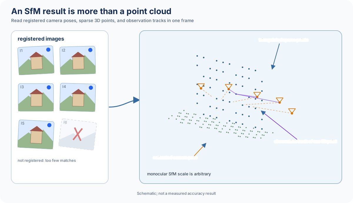
In a result viewer, first check whether cameras collapse into an implausibly small region, whether the point cloud splits or doubles, and whether any images failed to register. A building-like appearance alone does not demonstrate accuracy. Evaluate reprojection error, track length, and the number of registered images; when a surveyed length or GNSS is available, also compare against that external scale. Monocular SfM has an arbitrary global scale, so a distance shown by the point-cloud viewer is not automatically a distance in meters.
2. The Basic Pipeline
The earlier steps — feature extraction, matching, and geometric verification — are exactly the same elemental techniques covered in the Feature Detection Primer and the Epipolar Geometry Primer. SfM-specific design decisions come into play at the stage after each image-pair relationship has been found: how to assemble every image and every point into one consistent coordinate frame with no contradictions — which is where the two strategies of Incremental SfM and Global SfM diverge.
3. Incremental SfM: Adding Cameras One by One
Incremental SfM starts by choosing an initial image pair with sufficient parallax and enough correspondences, and building the first two-view reconstruction by estimating the Essential/Fundamental Matrix from epipolar geometry. From there, it repeats the following:
- Choose a new image that already has 2D correspondences to registered 3D points, and find that image's pose via PnP.
- Triangulate points not yet reconstructed in 3D, from correspondences between the new image and the existing ones.
- Refine pose and structure with local or global bundle adjustment every so many images.
- Return to step 1 until every image has been processed, or no more images can be added.
This approach, widely used since Snavely et al.'s Photo Tourism (2006), is also adopted by COLMAP's standard pipeline as Incremental SfM. Because it only increases a small number of unknowns at a time, sequentially, it's a robust implementation, and it's easy to detect and exclude a bad image pair. On the other hand, because poses are stacked up one image at a time, small errors early on propagate to later images, and datasets containing large loops (a group of images revisiting the same place) tend to accumulate drift. Periodic bundle adjustment, together with revisit detection equivalent to loop closure, is the key to keeping this accumulated error in check.
4. Global SfM: Solving All Pairwise Relationships at Once
Global SfM doesn't register images sequentially — it first finds the relative pose (R_{ij},\mathbf{t}_{ij}/\|\mathbf{t}_{ij}\|) for every (or a selected subset of) image pair. It then jointly estimates the whole graph in two stages.
Rotation averaging finds a globally minimally-inconsistent set of camera rotations \{R_i\} from the set of pairwise relative rotations R_{ij}. A commonly used error metric uses the logarithm map on the Lie group SO(3):
\rho is a robust loss, which suppresses the influence of wrong relative poses acting as outliers.
Translation averaging, once rotations are fixed, finds camera positions \{\mathbf{t}_i\} from the set of relative translation directions \mathbf{t}_{ij}. Since a monocular relative translation only gives a direction (see the scale ambiguity discussed in the Epipolar Geometry Primer), you need to solve for a consistent configuration from many pairwise directional constraints — approaches like 1DSfM, which include outlier removal, have been proposed for this.
Because Global SfM uses information from every image simultaneously, it's, in principle, less prone to the sequential drift that Incremental SfM sees, and it's also easier to parallelize computationally. But if outliers are mixed into individual relative poses, the whole global solution gets distorted unless they're detected and excluded at the averaging stage. Moulon et al.'s work (ICCV 2013) is a representative example that greatly improved Global SfM's practicality, combining robust rotation averaging with translation-direction estimation using the trifocal tensor.
| Aspect | Incremental SfM | Global SfM |
|---|---|---|
| How reconstruction proceeds | Adds one image at a time from an initial pair | Solves all pairwise relationships first, then optimizes jointly |
| Resistance to drift | Prone to sequential propagation and accumulated error | Little accumulated error since it's globally optimal |
| Resistance to outliers | Easy to detect and remove individually when adding an image | Outlier removal before averaging determines accuracy |
| Computational cost | Sequential in the number of images, tends to get heavy at large scale | Parallelizable, but requires global optimization for averaging |
| Implementation difficulty | Plenty of implementation examples, easy to tune for robustness | Theory and implementation of rotation/translation averaging are more difficult |
| Representative examples | Bundler, COLMAP (default), VisualSFM | openMVG (Global SfM pipeline), Theia |
In practice, rather than treating the two as a strict either/or, hybrid designs are also being researched — building a rough global pose with Global SfM and then refining it incrementally, or using only the high-confidence pairs in a Global fashion and adding the rest incrementally.
5. Triangulation and Track Management
Once poses are found for a group of images, triangulating corresponding points to obtain 3D points is itself an extension of the basic two-view geometry operation. What's SfM-specific is how to manage the correspondence, called a "track," when the same physical point is observed across three or more images.
- Because feature matching is done pairwise, matches between images A–B and B–C should, ideally, also imply a match between A–C, but in practice, this doesn't always hold given real descriptor distances. A trifocal consistency check guards the quality of tracks.
- The more observations a track contains, the more stable triangulation becomes, but a track composed only of images with small parallax between them still ends up with an unstable depth.
- Even a single wrong match mixed into a track doesn't just distort that point's 3D position — it also affects the residuals of the downstream bundle adjustment as a whole. RANSAC-style verification per track, and rejecting tracks with large reprojection error, are both necessary.
6. The Bridge to Bundle Adjustment
The pose and structure obtained from linear triangulation or sequential PnP are, at best, initial values. Simultaneously minimizing the reprojection error over all images —
— is Bundle Adjustment, and it's what ultimately determines SfM's final accuracy. Why this optimization has a sparse structure, and why the Schur complement makes it solvable even at large scale, are computational questions covered in depth in the Bundle Adjustment Primer. What's worth keeping in mind here is the difference in how it's used: Incremental SfM interleaves local bundle adjustment every few images added, while Global SfM runs a single full bundle adjustment once every global pose is in place.
7. Differences and Commonalities With Visual-SLAM
SfM and Visual-SLAM share the same mathematical tools — feature matching, epipolar geometry, PnP, and bundle adjustment. The difference lies in their goals and constraints.
| Aspect | Structure from Motion | Visual-SLAM |
|---|---|---|
| Processing style | Mostly offline batch processing | Online, real-time sequential processing |
| Input ordering | Can be unordered (any order, multiple cameras mixed in is fine) | Assumes chronologically continuous frames |
| Primary goal | High-quality 3D reconstruction prioritizing accuracy and completeness | Maintaining current self-position in real time |
| Optimization scope | Global bundle adjustment over all images is possible | Local/global optimization limited to keyframes, under strong compute-budget constraints |
| Handling revisits | Can verify every pair offline | Must detect and correct loop closure online |
| Representative implementations | COLMAP, openMVG, Bundler | ORB-SLAM family, VINS family |
In practice, combinations like using a high-precision 3D map built by SfM as SLAM's initial map or scale reference, or post-processing SLAM's keyframe trajectory offline with SfM to boost accuracy, are also common. The two aren't competing technologies — they complement each other across the offline/online time axis.
8. Representative Implementations
- COLMAP: centered on Incremental SfM, this is the currently most widely referenced research and production implementation, providing a consistent pipeline from feature extraction, matching, geometric verification, and reconstruction through to bundle adjustment and Multi-View Stereo.
- openMVG (open Multiple View Geometry): a library implementing both Incremental and Global SfM pipelines. Often paired with openMVS for dense reconstruction.
- Bundler: the pioneering Incremental SfM implementation that made the results of Photo Tourism public, and a comparison baseline for many subsequent works.
- Meshroom (AliceVision): an open-source photogrammetry tool with a GUI that handles everything from SfM through MVS to texturing in one pass.
When choosing a library, "newer means more accurate" isn't the right criterion — judge based on the number of images you're handling, GPU/CPU resources, the reliability of EXIF focal length, the matching strategy (exhaustive/sequential/vocabulary tree), and whether you want a single consistent pipeline all the way through MVS and texture generation.
9. Difficult Conditions and Common Failure Cases
- Texture-poor or highly repetitive scenes: uniform walls, tiled surfaces, and rows of crops in a field either yield no correspondences at all, or produce frequent mismatches.
- Sets of images with extremely small parallax: photos of a distant scene taken with a telephoto lens make triangulation unstable, leading to large depth errors.
- Moving objects and lighting changes: tourist-spot photo sets mix in people, vehicles, and seasonal or time-of-day differences, introducing correspondences that violate the static-scene assumption.
- Isolated image clusters: if shots split into two groups with no overlapping field of view, SfM can't unify them into one consistent coordinate frame, and reconstruction fragments into several disconnected pieces.
- Symmetric scenes: symmetric building facades, for instance, can converge to a geometrically consistent but physically wrong mirrored solution.
10. Practical Choices
- If shooting is fully ordered (video, or a robot's continuous frames), Incremental SfM's initial-pair selection becomes easy, and COLMAP's default pipeline is often enough.
- For large-scale image collections like internet tourist photos, where shooting order and overlap are both unknown, Global SfM's scalability tends to have the advantage.
- For applications requiring real-time performance (robots, AR, automotive), consider Visual-SLAM or VIO instead of SfM. SfM's main arena is offline, high-precision reconstruction.
- If you need a dense 3D shape (a mesh or textured model), start from SfM's sparse point cloud and pose, then move on to Multi-View Stereo.
11. Summary
Structure from Motion is a technology that jointly recovers camera poses and 3D structure, via feature matching and geometric verification, from an unordered set of images, using either the Incremental SfM or Global SfM strategy. Incremental is robust but prone to drift, and Global resists drift but is sensitive to outliers — a symmetric tradeoff. Under either strategy, final accuracy is carried by bundle adjustment, which connects directly onward to Visual-SLAM, its sibling technology operating on a different time axis, and to Multi-View Stereo, a dense-reconstruction technology.
Are reconstructed SfM distances automatically in meters?
Monocular reconstruction retains a scale ambiguity. Use known dimensions or positioning information to establish metric scale.
References
- Snavely, Seitz & Szeliski, Photo Tourism: Exploring Photo Collections in 3D (SIGGRAPH 2006)
- Schönberger & Frahm, Structure-from-Motion Revisited (CVPR 2016)
- Moulon, Monasse & Marlet, Global Fusion of Relative Motions for Robust, Accurate and Scalable Structure from Motion (ICCV 2013)
- Wilson & Snavely, Robust Global Translations with 1DSfM (ECCV 2014)
- COLMAP official documentation
- openMVG official documentation
- Hartley & Zisserman, Multiple View Geometry in Computer Vision (authors' official page)
Current step · 12 / 19 · Computer Vision Primer
Comments
Please log in to post a comment
No comments yet.