Contents — find the section you need
Background and reading guide
Background Basic vectors, matrices and camera projection.
Fundamentals · Includes code examples.
To judge whether two places in an image show the same thing, it's more efficient to compare small, repeatably findable cues than to compare the whole image. The process of selecting those cues is feature detection. It sits at the entry point of any process that needs correspondence between images — camera-motion estimation, panorama stitching, 3D reconstruction, image retrieval, visual inspection. This article separates "where to select" from "how to match the selected points," and organizes the thinking behind classical algorithms from both an equation and an implementation standpoint.
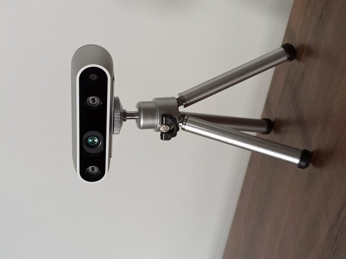 Intel RealSense D435
Image: Intel RealSense depth camera D435 (Marc Auledas, CC BY-SA 4.0), Wikimedia Commons. A representative camera, not a feature-detection-only device.

30-Second Summary
- Place feature points not on flat walls but at corners with intensity change in multiple directions, or at blobs whose brightness differs from their surroundings. Being re-detected at the same place after a small image transform (repeatability) is what matters.
- Corner detection captures the two-directionality of local gradients; blob detection captures a locally distinct patch of brightness at some scale. DoG quickly searches for blob candidates from the difference of multiple blurred images.
- FAST judges corners quickly by comparing only the pixels on a circle. ORB combines FAST with an image pyramid, orientation estimation, and a rotated BRIEF binary descriptor, suiting real-time use.
- SIFT selects scale via DoG, normalizes orientation with a gradient-direction histogram, and builds a 128-dimensional descriptor. Compute and memory cost rise, but it's robust to scale and rotation changes.
- Detection alone doesn't determine correspondence. Descriptor distance, the ratio test, and RANSAC-based geometric verification must be evaluated together as one pipeline. Recently, learning-based detection and matching such as SuperPoint, ALIKED, and LightGlue have also become practical.
What Is a Feature Point — Not "a Point That Stands Out" but "a Point You Can Find Again"
Let pixel coordinates be \mathbf{x}=(x,y)^\mathsf{T} and the image I(\mathbf{x}). A feature point is a location whose neighboring patch can be stably detected as the same physical location even after a slight translation, rotation, or scaling, and which can be distinguished from other points by the surrounding pattern. The former is called the detector, and whatever turns the latter into a numeric vector or bit string is called the descriptor.
These two are distinct. FAST is, in principle, a detector; BRIEF is a descriptor; ORB is a mechanism that combines both. SIFT is the combination of a DoG detector and a gradient-histogram descriptor. Comparing names alone invites confusion, so from here on we always treat this as three stages: "select points," "represent the surroundings," and "match points."
Figure: created by Duskcoil. System quality is governed not by the number of detections, but by the number of correspondences that end up geometrically consistent.
Corners: Selecting Places That Change in Two Directions
The most intuitive feature is the corner. Write the apparent change when an image patch W is shifted by a tiny displacement \mathbf{u}=(u,v)^\mathsf{T} as the SSD (sum of squared differences):
Under a first-order Taylor approximation, the local structure (second-moment) matrix \mathbf{M} becomes
where I_x,I_y are the image gradients and w is a weight such as a Gaussian window. Let \mathbf{M}'s eigenvalues be \lambda_1,\lambda_2; a point is a corner where even the smaller eigenvalue is large. At an edge, where gradient is large in only one direction, one eigenvalue stays small. In flat regions, both stay small. The Harris detector doesn't solve for eigenvalues explicitly at every pixel; instead it selects local maxima of the following response value:
k is typically around 0.04–0.06. Harris is relatively robust to rotation, but since it looks through a fixed-size window, it has no mechanism for selecting the same point when the subject is significantly enlarged or shrunk. Shi–Tomasi's \min(\lambda_1,\lambda_2) is also widely used as a practical criterion for selecting corners suited to tracking.
Blobs: A "Blob," Even Without a Corner, Is a Useful Cue
Corners alone don't adequately pick up round logos, spots, dark holes, or the center of a bright reflection. So a blob detector finds locally distinct patches of brightness relative to their surroundings, at some scale. Write the scale-space smoothed with a Gaussian G(\mathbf{x};\sigma) as
where * is convolution and \sigma represents "what size we're looking at." The scale-normalized response of the Laplacian of Gaussian (LoG),
responds strongly to a dark circle on a bright background, or a bright circle on a dark background. Finding extrema not just in position but in the three-dimensional (x,y,\sigma) space including the \sigma direction simultaneously picks out a blob's center and characteristic size. You can also interpret this as scale corresponding to a circular blob whose radius is approximately \sqrt{2}\sigma.
LoG is a great idea, but computing the exact second derivative at every scale is expensive. This approximation and speedup leads to DoG, and from there to SIFT.
DoG: Finding Scale-Invariant Candidates from a Difference of Blurs
The Difference of Gaussians (DoG) is the difference between two adjacent blurred images:
where k>1 is the ratio between adjacent scales. Up to a constant factor, DoG approximates the scale-normalized LoG, so blob candidates can be searched with just one extra convolution. In implementation, you build a Gaussian pyramid by progressively blurring the image, and compare each DoG pixel against its 8 neighbors at the same scale plus 9 neighbors each at the scale above and below — 26 total. A maximum or minimum makes it a candidate.
Candidates aren't used as-is. Weak extrema are noise and get rejected, as are extrema along elongated edges. Interpolating a 3D quadratic around a DoG extremum gives subpixel position and scale. For the Hessian
a large \mathrm{Tr}(\mathbf{H})^2/\det(\mathbf{H}) indicates an edge response where only one principal curvature is strong, and such points are excluded. This addresses the same problem as in corner detection: a point on an edge looks similar even when shifted along the edge, so its correspondence can't be pinned down uniquely.
FAST: Judging Corners Quickly by Looking Only at a Circle
Features from Accelerated Segment Test (FAST) uses the 16 pixels on a radius-3 Bresenham circle around pixel p. Given a threshold t, if n consecutive pixels (typically 9 or 12) are all brighter than I_p+t, or all darker than I_p-t, p is judged a corner.
Because it computes no gradients or matrices — just a small number of pixel comparisons plus early rejection — it's extremely fast. The design that first checks the pixels at the 1, 5, 9, and 13 o'clock positions on the circle, and immediately stops if a continuous run of bright/dark pixels can't possibly form, is key to its speed. On the other hand, plain FAST provides neither scale nor orientation, and tends to respond to many points along edges. Only after scoring the intensity difference from the surroundings, applying non-maximum suppression (NMS), and combining with an image pyramid does it become a practical multi-scale detector.
ORB: Not Leaving FAST as "Fast but Hard to Use"
ORB (Oriented FAST and Rotated BRIEF) is a construction that reinforces FAST and BRIEF, aimed at real-time image matching. First, it runs FAST across an image pyramid at each reduction ratio s, keeping the top points from each level. This gives, if not exact, robustness to scale change.
Next, it computes the intensity centroid of the patch around point p. From the moments
the angle \theta=\operatorname{atan2}(m_{01},m_{10}) from the center p to the centroid \mathbf{c} becomes the dominant orientation. The BRIEF descriptor is a bit string comparing pixel pairs (\mathbf{a}_i,\mathbf{b}_i) within the patch:
laid out roughly 256 times. In ORB, the point-pair coordinates are rotated by \theta before comparison, so the same bit pattern tends to result even after rotation. rBRIEF, which learns to select low-correlation comparison pairs, is another way of preserving the information content of the bits. Distance between binary strings can be computed quickly as the Hamming distance — the number of set bits after XOR.
ORB's strength is speed and memory efficiency on CPUs and embedded devices, and it's widely adopted in Visual SLAM. However, under large scale differences, heavy blur, or significant viewpoint change, SIFT or learning-based features with richer gradient descriptions can be advantageous.
SIFT: Consistently Normalizing Scale, Orientation, and Description
Scale-Invariant Feature Transform (SIFT) detects extrema of (x,y,\sigma) via DoG, and removes low-contrast points and edge responses. Around each point's neighborhood, it computes gradient magnitude and direction, and builds a Gaussian-weighted orientation histogram. The largest peak becomes the dominant orientation used to normalize the patch's rotation, and secondary peaks exceeding 80% of the max are also assigned their own orientation. This is the core of its robustness to rotation.
For the descriptor, a normalized window of roughly 16\times16 is divided into 4\times4 cells, and each cell gets an 8-direction gradient histogram. The dimensionality is therefore 4\times4\times8=128. The vector \mathbf{d} is L2-normalized, and elements exceeding 0.2 are clipped and renormalized, suppressing sensitivity to local lighting change.
In other words, SIFT's "invariance" isn't magic. It's an explicit design that addresses each source of variation individually: selecting scale via the image pyramid, rotating the coordinate frame by the dominant orientation, and absorbing contrast via normalization. It isn't complete against affine deformation or large viewpoint differences, which still require downstream RANSAC or multi-view geometry.
Minimal Implementation Pseudocode
Feature-point processing shouldn't stop at extraction — it should be implemented through to correspondence verification. Below is a skeleton that applies to either ORB or SIFT.
function match_images(imageA, imageB, method):
    grayA, grayB = to_gray(imageA), to_gray(imageB)
    detector = create(method)        # ORB: FAST+pyramid+rBRIEF / SIFT: DoG+gradient
    keyA, descA = detector.detect_and_compute(grayA)
    keyB, descB = detector.detect_and_compute(grayB)

    metric = HAMMING if method == ORB else L2
    tentative = []
    for each descriptor a in descA:
        b1, b2 = two_nearest(a, descB, metric)
        if distance(a, b1) < 0.75 * distance(a, b2):
            tentative.append((a.keypoint, b1.keypoint))

    H, inlier_mask = RANSAC_HOMOGRAPHY(tentative, reproj_threshold=3px)
    return tentative[inlier_mask], H
Taking only the single nearest neighbor leaves ambiguous points, such as window frames, grids, and repetitive patterns, in the result. Lowe's ratio test uses the ratio of the best distance d_1 to the second-best d_2, discarding candidates where the gap to the runner-up isn't large enough. RANSAC then estimates a homography \mathbf{H} or fundamental matrix from small random subsets of correspondences as a hypothesis, and picks the hypothesis that explains the most correspondences (inliers) with small reprojection error. If the object is planar, or the camera merely rotated in place, consistency can be checked with the homography
For a general 3D scene, the fundamental/essential matrix is used instead. The inlier count and ratio that survive to this point are the actually usable amount of feature.
What's Robust to Lighting, Scale, and Rotation, and to What Degree
Against lighting change, a simple brightness offset I'(x,y)=I(x,y)+b destroys pixel differences, but has little effect on the relative relationships in gradients or binary comparisons. A uniform contrast change I'=aI+b is also handled fairly well by SIFT's descriptor normalization. But when local structure itself changes — exposure saturation, shadow boundaries, reflections, day versus night — classical methods alone offer no guarantees. During capture, fix or tightly manage exposure, and if needed, apply local contrast correction such as CLAHE under the same conditions to both images. Over-correction risks turning noise into spurious features, so be careful.
Single-resolution Harris or FAST is inherently weak against scale change. ORB, which searches candidates across an image pyramid, has practical tolerance, though not the same normalization as SIFT, which selects continuous scale extrema via DoG. If texture disappears at reduced scale, no method can find correspondence. Input resolution, pyramid depth, and minimum patch size should be decided from the expected range of capture-distance variation.
Against rotation, the Harris response itself is relatively stable, but matching requires rotating the descriptor's coordinate frame as well. ORB assigns orientation via the intensity centroid, SIFT via the gradient-direction histogram. Such continuous-angle normalization is more effective than a descriptor that only handles 90-degree rotation steps. Meanwhile, a strong oblique view isn't rotation-and-scaling but an affine/projective deformation, calling instead for multi-view data, affine-covariant features, or learning-based features combined with geometric verification.
Evaluation Metrics: Measure Usable Correspondences, Not Point Count
For an image pair with a known homography H, project point \mathbf{x}_i from image A into B, and if a point within distance \epsilon exists in the detected point set K_B, count it as a successful re-detection. Repeatability is conceptually
But finding the same location is useless if the descriptors can't distinguish it. So you also report matching precision (fraction of correct correspondences), correct-correspondence count, post-RANSAC inlier ratio, rotation/translation error of the estimated pose, processing time, and memory. HPatches is a representative benchmark that separates lighting change from viewpoint change to evaluate patch matching, detectors, and homography estimation. Unless you measure with data matching your application's geometry (planar, or wide-baseline 3D), you shouldn't adopt a single score's ranking as-is.
| Method | Detection core | Descriptor | Scale/rotation | Matching distance | Strengths | Main caveats |
|---|---|---|---|---|---|---|
| Harris + patch | Structure matrix | Raw patch, etc. | Scale ✕, rotation separate | SSD/NCC | Clear principle | Weak to lighting/scale |
| LoG / DoG | Scale-space blob extrema | Needs separate descriptor | Scale ◎, rotation separate | Depends on descriptor | Gets blob and scale | Pyramid computation required |
| FAST + BRIEF | Continuous brightness on circle | Binary comparison | Neither alone | Hamming | Very fast | Weak to viewpoint/scale |
| ORB | Pyramid FAST | Rotated rBRIEF | Scale ○, rotation ○ | Hamming | Lightweight, real-time-friendly | Limited under large deformation |
| SIFT | DoG extrema | 128-dim gradient histogram | Scale ◎, rotation ◎ | L2 | Solid, well-validated | CPU/memory heavy |
| Learning-based | Learned via network | Learned vector | Strengthened via data | L2 / learned | High correspondence rate in hard conditions | Needs model, GPU, reproducibility management |
The table's ○ and ◎ are not absolute ratings — they're relative benchmarks for typical implementations and expected ranges. Even SIFT is ambiguous when the same grid pattern fills the frame, and even ORB can obtain enough inliers under moderate conditions.
Where This Sits in Current Libraries and Real Products
For a first prototype, OpenCV's cv::ORB::create(), cv::SIFT::create(), and cv::FastFeatureDetector::create() are easy to work with. ORB pairs with BFMatcher(NORM_HAMMING); SIFT with an L2-distance BFMatcher or a FLANN-based matcher. Even if you want detector and descriptor separated, OpenCV's Feature2D API keeps you on the same flow. For learning-based experimentation and GPU processing, Kornia on PyTorch provides SIFT, ORB, DISK, KeyNet/HardNet, LightGlue, and more as building blocks.
In photogrammetry and 3D reconstruction practice, COLMAP is the representative tool; its current official documentation supports standard SIFT plus ALIKED when built with ONNX enabled. Since both SIFT and ALIKED can connect to either brute-force matching or LightGlue matching, it's easy to compare classical and learning-based approaches at the reconstruction entry point. When choosing a product or library, it's better to first decide whether it must run CPU-only, the latency budget, whether heavy offline matching is acceptable, and whether reproducible version pinning is required — rather than whether the model name sounds new.
Recent Research: Jointly Optimizing Detection, Description, and Matching
One turning point for learning-based approaches was SuperPoint. A fully convolutional network outputs an interest-point probability map and a descriptor map at once, learning self-supervised, via Homographic Adaptation, to reproduce points across geometric transforms. This is the idea of learning from data where correspondence-useful locations are, rather than relying solely on a hand-designed notion of "corner-ness."
DISK addresses the problem that selecting sparse points and matching them is discrete and hard to differentiate, by optimizing detection and description end-to-end with policy gradients that reward correct correspondence count. ALIKED uses a Sparse Deformable Descriptor Head that learns deformable support locations around each keypoint, aiming to balance expressiveness and efficiency by extracting descriptors at sparse points rather than from the whole dense feature map.
Matchers, too, are shifting away from independent nearest-neighbor search. LightGlue estimates correspondences between two sets of local features using an attention mechanism, with adaptive computation that stops early when an image pair is easy. This isn't a feature detector itself, but it's an important reminder that good descriptor distance from the detector alone doesn't guarantee good final correspondences. Currently, it's practical to compare a setup using classical features with a lightweight matcher against a setup matching learned features like SuperPoint/ALIKED with LightGlue, under identical RANSAC settings on your target data.
Selection and Tuning Checklist
- First, log detection count, ratio-test pass count, RANSAC inlier count, inlier ratio, and processing time on real image pairs. Increasing detection count alone can backfire if mismatches increase along with it.
- For short-duration tracking near a fixed camera, start with FAST/ORB and tune
nfeatures, the FAST threshold, and pyramid levels. Under low texture, check blur, exposure, and focus before lowering the threshold. - For matching still images with large changes in capture distance or rotation, use SIFT as the baseline. Whether a faster method beats SIFT must always be verified on the same data with the same geometric verification.
- At night, under strong backlight, across seasonal change, or with wide viewpoint differences, also consider learning-based features. But include the gap between training data and the target environment, model updates, and GPU availability in the performance evaluation.
- Repetitive patterns, specular surfaces, moving objects, and extreme motion blur are less a feature-detection problem than an observation ambiguity. Compensate with masking, temporal tracking, sensor fusion, and capture planning.
Feature detection isn't an all-purpose classifier for understanding images. But it remains an effective foundational technology for selecting, with little compute, which pixels can support geometry. Understanding the ideas of corners, blobs, scale space, and orientation normalization lets you trace the failure causes behind the numbers, whether you're tuning classical ORB/SIFT or evaluating learning-based features.
Is every point on a strong edge easy to track?
Motion along a single edge is ambiguous. Corners provide intensity changes in different directions, making two-dimensional motion easier to identify.
References
- Lowe, Distinctive Image Features from Scale-Invariant Keypoints (SIFT original paper, IJCV 2004)
- Rublee et al., ORB: an efficient alternative to SIFT or SURF (ICCV 2011)
- OpenCV Feature2D / ORB class reference
- OpenCV SIFT class reference
- OpenCV FAST Feature Detector tutorial
- HPatches: benchmark and evaluation of handcrafted and learned local descriptors (CVPR 2017)
- SuperPoint (CVPR Workshops 2018)
- DISK (NeurIPS 2020)
- ALIKED (arXiv 2023)
- LightGlue (ICCV 2023)
- COLMAP Feature Extraction and Matching documentation
- Kornia feature module documentation
Current step · 2 / 19 · Computer Vision Primer
Comments
Please log in to post a comment
No comments yet.