Bundle Adjustment Primer — the Nonlinear Least Squares That Polish Camera Poses and 3D Points Together

The camera poses and 3D points that Structure from Motion and Visual-SLAM obtain via triangulation and PnP are, at best, rough initial values from linear approximations and sequential processing. Per-image noise, quantization error in correspondence points, and propagated error from sequential estimation all pile up, leaving a reconstruction that's internally inconsistent as it stands. Bundle Adjustment (BA) is the final polishing optimization that resolves this inconsistency by moving every camera parameter and every 3D point at once, minimizing the sum of reprojection error across all observed points. The name "bundle" comes from adjusting the bundle of light rays running from each 3D point to each camera, all at once, so they agree with the observed positions.

0. 30-Second Summary

Bundle Adjustment is a nonlinear least-squares problem whose unknowns are the cameras' intrinsic/extrinsic parameters and the 3D-point coordinates, minimizing the sum of squared reprojection error over all observations.
It's solved iteratively with the Gauss-Newton method or Levenberg-Marquardt (LM). LM smoothly interpolates, via a parameter $\lambda$ , between the unstable-but-fast Gauss-Newton method and the slow-but-stable steepest-descent method.
Since a single camera is only ever linked to the points it actually saw, the Jacobian and the Hessian approximation take on a sparse, block-structured form organized by camera × point. This sparsity is the key that makes large-scale problems tractable.
The Schur complement trick exploits the fact that the 3D-point blocks are mutually independent (block-diagonal), eliminating the points first to solve a small "reduced camera system" involving only the cameras. This is what makes it possible to solve problems at the scale of tens of thousands of points and thousands of cameras in realistic time.
Bundle Adjustment is a close relative of SLAM's Pose Graph optimization, differing in that its unknowns include the 3D points themselves. It's a shared foundational technology, used both to finish off SfM and for SLAM's local/global optimization.

1. What Does It Take as Input, and What Does It Solve For?

The input consists of the following three initial estimates, obtained as intermediate results from SfM or Visual-SLAM:

Initial values for camera poses $\{K_i, R_i, \mathbf{t}_i\}$ ( $i=1,\dots,m$ ; in many cases the intrinsic parameters $K_i$ are known or fixed)
Initial values for 3D points $\{\mathbf{X}_j\}$ ( $j=1,\dots,n$ ; rough coordinates obtained from triangulation)
The correspondence of which camera observed which point — that is, the image coordinates $\mathbf{u}_{ij}$ for each observation (the pixel position at which camera $i$ saw point $j$ )

The output is camera poses and 3D points, all finely adjusted simultaneously, that are more internally consistent across every observation. The fact that Bundle Adjustment isn't a method for building a solution from scratch, but rather a finishing optimization that locally polishes an already "roughly correct" initial value, matters for the discussion of convergence below.

2. The Cost Function: Reprojection Error

The mismatch between where a 3D point $\mathbf{X}_j$ projects into camera $i$ and the actually observed image coordinate $\mathbf{u}_{ij}$ is called the reprojection error. Writing camera $i$ 's pose as $R_i, \mathbf{t}_i$ and the projection function as $\pi(\cdot)$ (the nonlinear map converting homogeneous coordinates into pixel coordinates), the residual for one observation is

r_{ij} = \pi\big(K_i(R_i\mathbf{X}_j + \mathbf{t}_i)\big) - \mathbf{u}_{ij}

Bundle Adjustment minimizes the sum of squares of this residual over the entire set of observed pairs $\mathcal{O}=\{(i,j)\}$ .

\min_{\{K_i,R_i,\mathbf{t}_i,\mathbf{X}_j\}}\sum_{(i,j)\in\mathcal{O}}\rho\left(\|r_{ij}\|^2\right)

$\rho$ is a robust loss function such as the Huber loss, which prevents a single large outlier from a mismatch from distorting the entire optimization. This equation is exactly the same form already seen in the SfM Primer — Bundle Adjustment deals with the computational core of actually solving this minimization problem.

3. Solving as Nonlinear Least Squares: From Gauss-Newton to Levenberg-Marquardt

Collecting every unknown into a single vector $\mathbf{x}$ (all camera poses and all 3D points laid out together), and writing the whole set of residuals as $\mathbf{r}(\mathbf{x})$ , the minimization target is $\|\mathbf{r}(\mathbf{x})\|^2$ . Since $\mathbf{r}$ is nonlinear, we use a first-order Taylor expansion around the current estimate $\mathbf{x}_k$ : $\mathbf{r}(\mathbf{x}_k+\Delta\mathbf{x})\approx \mathbf{r}(\mathbf{x}_k)+J\Delta\mathbf{x}$ . $J=\partial \mathbf{r}/\partial \mathbf{x}$ is the Jacobian. Substituting this in and solving for $\Delta\mathbf{x}$ gives the Gauss-Newton method's normal equation:

(J^\mathsf{T}J)\,\Delta\mathbf{x} = -J^\mathsf{T}\mathbf{r}

$H=J^\mathsf{T}J$ is the Hessian approximation (the Gauss-Newton approximation, ignoring second-order terms). Solving this equation for $\Delta\mathbf{x}$ , updating $\mathbf{x}_{k+1}=\mathbf{x}_k+\Delta\mathbf{x}$ , and repeating this operation until the residual converges is the whole procedure.

The Gauss-Newton method converges fast when the initial value is close to the solution, but tends to diverge with a poor initial value. Levenberg-Marquardt (LM), proposed independently by Levenberg (1944) and Marquardt (1963), eases this by adding a damping term to the normal equation.

(J^\mathsf{T}J + \lambda D)\,\Delta\mathbf{x} = -J^\mathsf{T}\mathbf{r}

$D$ is usually the diagonal of $J^\mathsf{T}J$ (or an equivalent scaling matrix), and $\lambda$ is the damping coefficient. When $\lambda$ is small, this behaves close to Gauss-Newton and converges fast; when $\lambda$ is large, it takes small, safe steps closer to steepest descent. Through an adaptive control scheme — shrink $\lambda$ to accelerate whenever the cost decreases each iteration, and grow $\lambda$ to reject and shorten the step whenever the cost increases — LM bridges Gauss-Newton's speed with steepest descent's stability. Nearly every practical implementation of Bundle Adjustment (Ceres Solver, g2o, SBA, and others, discussed below) adopts LM or a closely related trust-region method.

4. Why Is the Jacobian Sparse?

Bundle Adjustment's unknowns are camera pose (6 degrees of freedom — 3 rotation plus 3 translation, if intrinsic parameters are fixed) × $m$ cameras, and 3D point (3 degrees of freedom) × $n$ points, adding up to as many as $6m+3n$ dimensions. In real SfM problems with tens of thousands of observations or more, naively treating this $J^\mathsf{T}J$ as a dense matrix costs $O((6m+3n)^3)$ — not solvable in realistic time.

What comes to the rescue here is the structure that the reprojection error $r_{ij}$ "depends only on camera $i$ 's parameters and point $j$ 's parameters." The partial derivatives with respect to any other camera $k\neq i$ or point $l\neq j$ are identically zero.

\frac{\partial r_{ij}}{\partial \mathbf{x}_{\text{camera }k}} = 0 \ (k\neq i), \qquad \frac{\partial r_{ij}}{\partial \mathbf{X}_l} = 0 \ (l\neq j)

In other words, the row of the Jacobian generated by a single observation has nonzero entries only in the block for the corresponding camera and the block for the corresponding point. The number of rows grows in proportion to the number of observations, but the number of nonzero entries per row stays constant (camera 6 + point 3, or a bit more if intrinsic parameters are included). This sparsity shows up, when you look at $J^\mathsf{T}J$ , as the following block structure.

J^\mathsf{T}J = \begin{pmatrix} B & E \\ E^\mathsf{T} & C \end{pmatrix}

$B$ : interactions among camera parameters. This is zero unless cameras $i$ and $k$ observe a common point, so it has a sparse block structure.
$C$ : interactions among 3D-point parameters. Since one point $j$ 's 3 degrees of freedom are never coupled to any other point, this is a block-diagonal matrix — the premise for the Schur complement trick in the next section.
$E$ : interactions between cameras and points (a nonzero block appears for each observation $(i,j)$ ).

5. The Basic Pipeline

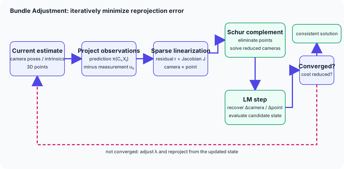
$r_{ij}$ Sparse Jacobiancamera × pointblock structure Eliminate points viaSchur complement,reduced camera system Adjust $\lambda$ viaLM method,update $\Delta\mathbf{x}$ Checkconvergence

Every iteration recomputes the reprojection error, assembles the sparse Jacobian, solves the camera-only reduced system via the Schur complement, and updates via LM's step control. This repeats until the change in cost drops below a threshold, or until a maximum number of iterations is reached.

6. The Schur Complement Trick: Turning Sparsity Into Reduced Computation

Using the block structure from the previous section, we can write the normal equation $(J^\mathsf{T}J+\lambda D)\Delta\mathbf{x}=-J^\mathsf{T}\mathbf{r}$ split into the camera update $\Delta\mathbf{c}$ and the point update $\Delta\mathbf{p}$ as

\begin{pmatrix} B' & E \\ E^\mathsf{T} & C' \end{pmatrix} \begin{pmatrix} \Delta\mathbf{c} \\ \Delta\mathbf{p} \end{pmatrix} = \begin{pmatrix} v \\ w \end{pmatrix}

(where $B', C'$ are the blocks after adding the damping term). Since $C'$ is a block-diagonal matrix, independent per 3D point, each 3×3 block can be inverted individually, at a cost roughly proportional to the number of points $n$ . Using this $C'^{-1}$ to eliminate $\Delta\mathbf{p}$ leaves the reduced camera system, involving cameras only:

\left(B' - E C'^{-1}E^\mathsf{T}\right)\Delta\mathbf{c} = v - E C'^{-1}w

The left-hand side's $B'-EC'^{-1}E^\mathsf{T}$ is called the Schur complement. This matrix has size $6m\times 6m$ (depending only on the number of cameras, not on the number of points $n$ ), and once $\Delta\mathbf{c}$ has been solved, each point's update can be cheaply recovered with

\Delta\mathbf{p} = C'^{-1}\left(w - E^\mathsf{T}\Delta\mathbf{c}\right)

In a typical SfM problem, the number of points $n$ can be dozens of times the number of cameras $m$ , so instead of naively solving a system with $6m+3n$ dimensions, you only need to handle the Schur complement, of dimension $6m$ . This is the core idea that makes Bundle Adjustment practically solvable even at the scale of tens of thousands of points. It was theoretically organized by Triggs et al.'s "Bundle Adjustment — A Modern Synthesis" (2000), and it's the standard internal implementation in current libraries like Ceres Solver and g2o.

Ceres Solver offers multiple options just for how to solve this reduced system: DENSE_SCHUR, which solves it as a dense matrix (up to a few hundred cameras); SPARSE_SCHUR, which exploits sparsity via reordering (thousands of cameras); and ITERATIVE_SCHUR, which applies conjugate gradient to the Schur complement (for even larger-scale problems). Choosing among these based on the scale of the problem is a practical rule of thumb.

7. Gauge Freedom: the Directions Along Which the Solution Isn't Uniquely Determined

Bundle Adjustment retains a degree of freedom that can move the whole set of parameters without changing the value of the cost function. Moving every camera and every 3D point together by the same rotation, translation, and scale leaves the reprojection error completely unchanged (for a monocular-only case, absolute scale is likewise indeterminate). This degree of freedom is called gauge freedom. Left unaddressed, it makes $J^\mathsf{T}J$ singular (rank-deficient), which either makes the normal equation unsolvable, or numerically unstable.

In practice, this is worked around by fixing the pose of the first two cameras or one baseline length, or by relying on the fact that LM's own damping term $\lambda D$ implicitly regularizes this singular direction. When absolute-scale or absolute-pose information is available — from GPS or an IMU, say — it's natural to use that as an additional constraint to fix the gauge.

8. The Difference From Pose Graph Optimization

Pose Graph optimization, covered in the Loop Closure Primer, also belongs to the same mathematical framework as Bundle Adjustment in the sense that it minimizes, with a robust loss, a nonlinear least-squares residual built with the $\mathrm{Log}$ map. The difference lies in what the unknowns actually are.

Aspect	Bundle Adjustment	Pose Graph Optimization
Unknowns	Every camera pose + every 3D-point coordinate	Every camera's (node's) pose only
Residual	3D-point reprojection error (image space)	Difference from relative-pose observations ( $SE(3)$ space)
Source of sparsity	Which camera saw which point	Which node pairs are linked by a constraint
Computational cost	High with many points, tamed via the Schur complement	Inherently smaller, scaling with the number of nodes (keyframes)
Primary use	Final polish of SfM, refining local/global maps	Global drift correction in SLAM (after loop closure)

In actual Visual-SLAM systems, it's common to see a division of labor: local bundle adjustment (local BA), including 3D points, refines the area around keyframes on a per-frame basis, while lightweight Pose Graph optimization without explicit 3D points quickly corrects the global trajectory whenever a loop closure is detected. Full bundle adjustment including 3D points (global BA) is more accurate but computationally costly, so it can't be run frequently in situations that demand real-time performance.

9. Representative Implementations

Ceres Solver: a general-purpose nonlinear least-squares library developed by Google, in production use since 2010. It has Schur-based solvers built in, and is used as the bundle-adjustment backend for many SfM/SLAM implementations, including COLMAP.
g2o: a graph-optimization framework published by Kümmerle et al. at ICRA 2011, capable of handling both SLAM's Pose Graph optimization and bundle adjustment within the same framework. It has been widely used as the backend of the ORB-SLAM family.
SBA (Sparse Bundle Adjustment): an early publicly available implementation specialized for sparse bundle adjustment, published by Lourakis and Argyros in ACM Transactions on Mathematical Software in 2009. It's often referenced as a representative example that explicitly implements the Schur complement trick.
COLMAP's built-in BA: internally uses Ceres Solver, automatically switching between local and global bundle adjustment at each step of Incremental SfM.

10. Difficult Conditions and Common Failure Cases

Poor initial values: Bundle Adjustment is a local optimization — if the initial value is far from the true solution, it can converge to the wrong local solution, or fail to converge at all. The quality of the initial value obtained from triangulation or PnP determines the final accuracy.
Points with few observations or small parallax: a point observed from only a very small number of images, or with little parallax, tends to have an ill-conditioned Jacobian, and can leave a large residual error concentrated purely along the depth direction.
Heavy outlier contamination: with many mismatches mixed in, even a robust loss can't fully absorb them, and correct neighboring points can end up dragged and distorted too.
Extremely large-scale problems: for city-scale reconstructions with observation counts running into the millions, even with the Schur complement, compute and memory costs become non-negligible, requiring the problem to be split and parallelized, or combined with approximate techniques (such as coarsening LM's trust region).
Unhandled gauge freedom: as noted above, forgetting to fix the gauge causes numerical instability, leading to failure to converge, or wandering into a non-physical solution.

11. Practical Choices

If you need dense accuracy as the final stage of SfM, running a full bundle adjustment at the end — regardless of whether you used Incremental or Global strategy — is the standard rule. Following the default settings of an existing implementation like COLMAP is unlikely to lead you far astray.
For real-time SLAM, full bundle adjustment on every single frame is too computationally expensive. A practical design combines local bundle adjustment over just the most recent set of keyframes, with Pose Graph optimization that only fires on loop closure.
If you're building your own pipeline from scratch, it's reasonable to build it on top of a library like Ceres Solver or g2o. Writing a Schur-complement implementation from zero brings little learning benefit relative to the cost of verifying its correctness.
For large-scale, city-scale reconstruction, rather than relying on a single bundle adjustment, consider methods that split the problem by region and integrate hierarchically (this is also commonly done as a preliminary stage feeding into Multi-View Stereo, discussed below).

12. Summary

Bundle Adjustment is a nonlinear least-squares problem that simultaneously minimizes reprojection error across every camera and every 3D point, solved iteratively via the Levenberg-Marquardt method. The Schur complement trick, which exploits the sparsity of the camera-point observation relationship, is what makes this optimization solvable in realistic time even at the scale of tens of thousands of points. While it shares a mathematical framework with Pose Graph optimization, the choice between the two comes down to whether 3D points are explicitly held, and it's a shared foundational technology that ultimately underpins the accuracy of both SfM and SLAM.

References

#Bundle Adjustment #Nonlinear Least Squares #Levenberg-Marquardt #Schur Complement #Structure from Motion

References

- Triggs, McLauchlan, Hartley & Fitzgibbon, Bundle Adjustment — A Modern Synthesis (Vision Algorithms: Theory and Practice, 2000)
- Kümmerle, Grisetti, Strasdat, Konolige & Burgard, g2o: A General Framework for Graph Optimization (ICRA 2011)
- Lourakis & Argyros, SBA: A Software Package for Generic Sparse Bundle Adjustment (ACM Transactions on Mathematical Software, 2009)
- Ceres Solver official documentation: Non-linear Least Squares
- Ceres Solver official documentation: Schur-Based Linear Solvers
- Hartley & Zisserman, Multiple View Geometry in Computer Vision (authors' official page)
Current step · 13 / 19 · Computer Vision Primer
Comments
Please log in to post a comment
No comments yet.