Contents — find the section you need
Change parameters and verify
Open the panel, then press Run to load Python. You can stop execution and reset parameters. Results are computed on this device. No Python installation is required.
Local execution steps below are optional for reproducing the source results; they are not required for the browser experiment.
The experiment controls are in English.
Compare voltage drops in your browser
The panel above contains two independent arithmetic exercises, with synthetic curves and A/B comparison. No equipment or local Python installation is required. The original measurement procedure below remains optional; these curves do not diagnose a particular robot.
Supply path: an ideal source feeds battery resistance, then shared wiring/contact resistance, then an imposed total current. Shared resistance includes the outgoing and return paths. Battery-terminal voltage is Vs − I Rbattery; converter-input voltage is Vs − I (Rbattery + Rshared). The imposed current starts at 2 A, rises by the selected extra current at 0 ms, and returns at 100 ms. Repeated time coordinates show the left and right limits of the ideal steps. This is an algebraic resistance model, with no inductance, battery chemistry, charge state, current limiting or motor dynamics. Converter output, computer voltage and reset thresholds are not modeled. The current is prescribed, not calculated from a regulated constant-power load.
The defaults split the article's assumed 0.12 Ω into 0.04 Ω battery and 0.08 Ω shared resistance. An extra 5 A therefore adds 0.6 V of converter-input drop. Baseline resistance losses remain present: the 7 A plateau gives 11.72 V at the battery terminals and 11.16 V at the converter input from a 12 V ideal source. Move the resistance between the two segments while keeping the total fixed: the same downstream dip can have different battery-terminal evidence. This demonstrates measurement-point dependence, not a unique real fault diagnosis.
Separate capacitor exercise: a hypothetical capacitor alone supplies a constant missing current for the selected duration. Charge-related droop is I × t / C; terminal droop during discharge is I × ESR + I × t / C. Capacitance is entered in mF (50 mF = 0.05 F = 50,000 µF), time in ms. Time zero on this plot means just after discharge begins, so nonzero ESR gives an immediate drop. The plot stops just before the current ends: recharge and the end-of-discharge ESR recovery are not simulated. Initial capacitor voltage is unspecified; the graph shows voltage change, not a remaining supply voltage. It does not assert that any selected droop is physically usable with a particular starting voltage or load.
The default 1 A, 10 ms, 50 mF and zero ESR reproduce the article's ideal 0.2 V example. Halving capacitance doubles only the charge term; adding ESR adds its own step. The capacitor is not connected to the supply-path model. Changing capacitor settings cannot improve the upper curve. No converter-loop response, ESL, inrush, ripple rating, temperature, tolerance, stability or component recommendation is included. Slider bounds are teaching choices, not equipment ratings.
The data table includes both sides of supply steps and every capacitor sample. A/B uses common axes within each panel; the panels describe different experiments and time intervals. All outputs are synthetic calculations, not measurements or successful-start evidence. Use actual component documentation and the original measurement procedure for real fault isolation.
References: Analog Devices: real-source resistance model and TI: capacitance, ESR and transient behavior, reviewed 2026-09-20. This Lab applies Ohm's law and the constant-current capacitor relation under the assumptions above; it does not reproduce either source's hardware experiment or converter design. For energy sampling, see the separate power-measurement Lab.
यदि मोटर चालू होने पर कंप्यूटर रीसेट हो जाता है, तो पावर पाथ और सॉफ़्टवेयर लॉग की जाँच करें। पर्याप्त नाममात्र बैटरी वोल्टेज कनवर्टर या कंप्यूटर पर पर्याप्त क्षणिक वोल्टेज की गारंटी नहीं देता है। यह प्रक्रिया कम वोल्टेज वाले डीसी मोबाइल रोबोटों के लिए है, न कि मेन या उच्च वोल्टेज ट्रैक्शन सिस्टम के लिए।
पावर पाथ बनाएँ
बैटरी, सुरक्षा, कनेक्टर, वायरिंग, डीसी-डीसी कनवर्टर और कंप्यूटर का मानचित्र बनाएँ। उन अनुभागों को चिह्नित करें जो मोटर और कंप्यूटर दोनों की धारा प्रवाहित करते हैं, जिसमें रिटर्न कंडक्टर भी शामिल हैं। बैटरी, एक्चुएटर और डीसी-डीसी कनवर्टर को अलग-अलग समझना साझा प्रतिबाधा की जाँच का विकल्प नहीं है।
नाममात्र वोल्टेज लोडेड वोल्टेज से भिन्न होता है
कुल बैटरी, वायरिंग और संपर्क प्रतिरोध 0.12 Ω और स्टार्टअप के दौरान अतिरिक्त 5 A मान लें। अतिरिक्त प्रतिरोधक अवक्षेप \Delta V=\Delta I R=0.6 V है। यह एक काल्पनिक उदाहरण है, किसी विशिष्ट रोबोट के लिए मापा गया प्रतिरोध नहीं। वायरिंग इंडक्टेंस और कनवर्टर प्रतिक्रिया समय-निर्भर प्रभाव डालते हैं।
केवल बैटरी पर माप लेने से आगे की वायरिंग में होने वाले नुकसान छूट सकते हैं। वास्तविक मॉडल के न्यूनतम इनपुट वोल्टेज और आपूर्ति स्थितियों की जाँच करें; उदाहरण के लिए, रास्पबेरी पाई दस्तावेज़ीकरण मॉडल-विशिष्ट आवश्यकताओं को स्पष्ट करता है।
एक समयरेखा पर अवक्षेप का पता लगाएं
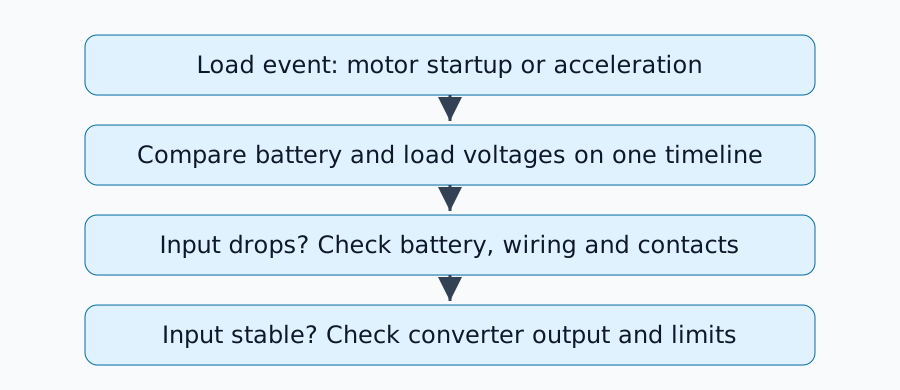
लोड इवेंट, बैटरी चार्ज, वायरिंग और उपकरण संस्करणों को ठीक करें। जहां संभव हो, बैटरी टर्मिनलों, कनवर्टर इनपुट, कनवर्टर आउटपुट और कंप्यूटर टर्मिनलों को एक साथ देखें। औसत मल्टीमीटर डिस्प्ले छोटे अवक्षेपों को नज़रअंदाज़ कर सकता है।
ऑसिलोस्कोप से, प्रोब रेटिंग और ग्राउंडिंग की जाँच करें ताकि कनेक्शन सर्किट को शॉर्ट न कर दे। ऐसे सर्किट की जांच न करें जिसकी ग्राउंडिंग आप स्थापित नहीं कर सकते; एक उपयुक्त विभेदक मापन विधि चुनें। कम वोल्टेज डीसी साइड पर माप लेते रहें और सुरक्षा सर्किट को निष्क्रिय न करें।
अगले जाँच चरण का चयन करने के लिए प्रेक्षणों का उपयोग करें
| प्रेक्षण | संभावित कारण | अगली जाँच |
|---|---|---|
| बैटरी वोल्टेज में गिरावट | आंतरिक प्रतिरोध, चार्ज या करंट सीमाएँ | विनिर्देशों के साथ मिलान लोड स्थितियों की तुलना करें |
| बैटरी स्थिर, कनवर्टर इनपुट में गिरावट | वायरिंग या संपर्क | प्रत्येक खंड में वोल्टेज में गिरावट |
| इनपुट स्थिर, कनवर्टर आउटपुट में गिरावट | करंट सुरक्षा, क्षणिक प्रतिक्रिया या इनपुट सीमाएँ | डेटाशीट और लोड स्टेप |
| कनवर्टर आउटपुट स्थिर, कंप्यूटर इनपुट में गिरावट | अंतिम केबल या कनेक्टर | लोड टर्मिनलों पर वोल्टेज |
तालिका परिकल्पनाओं को सीमित करती है; एक तरंगरूप किसी विशिष्ट कारण को स्थापित नहीं करता है। यदि आपूर्ति वोल्टेज मान्य रहता है, तो संचार, रीसेट सिग्नल, तापमान और सॉफ़्टवेयर की जाँच करें।
कैपेसिटर लगाना ही एकमात्र समाधान नहीं है
आदर्श डिस्चार्ज संबंध C=I\Delta t/\Delta V का उपयोग करते हुए, 0.2 V ड्रॉप के भीतर 10 ms के लिए अतिरिक्त 1 A की आपूर्ति के लिए C=0.05 F, या 50,000 µF की आवश्यकता होती है। यह मानकर चला जा रहा है कि कैपेसिटर सभी अनुपलब्ध करंट की आपूर्ति करता है और इस मान को स्थापित करने की अनुशंसा नहीं की जाती है। ESR, इनरश करंट और कनवर्टर स्थिरता भी मायने रखती हैं।
घटक जोड़ने से पहले, साझा वायरिंग प्रतिरोध, संपर्क और कनवर्टर की परिचालन सीमा की जाँच करें। प्रासंगिक घटक डेटाशीट और क्षणिक विशिष्टताओं को खोजने के लिए TI के पावर-मैनेजमेंट दस्तावेज़ जैसे संसाधनों का उपयोग करें।
समान परिस्थितियों में दोहराएँ
संशोधन, न्यूनतम स्टार्टअप वोल्टेज, रीसेट, परीक्षण गणना और बैटरी स्थिति रिकॉर्ड करें। एक सफल रन सभी चार्ज स्थितियों और एक साथ लोड पर सफलता की गारंटी नहीं है।
प्रत्येक परीक्षण के लिए एक पंक्ति का उपयोग करें ताकि एक सफल शुरुआत एक आंतरायिक रीसेट को न छिपाए। समान स्टार्टअप अंतराल पर न्यूनतम वोल्टेज रिकॉर्ड करें; यदि चैनलों को अलग-अलग परीक्षणों में मापा गया है, तो उन्हें एक साथ तरंगरूप के बजाय अलग-अलग माप के रूप में चिह्नित करें।
| परीक्षण / परिवर्तन | बैटरी की स्थिति / एक साथ लोड | बैटरी न्यूनतम (V) | कनवर्टर इनपुट / आउटपुट न्यूनतम (V) | कंप्यूटर न्यूनतम (V) | रीसेट / अवलोकन |
|---|---|---|---|---|---|
| परिवर्तन से पहले / परीक्षण 1 | रिकॉर्ड करने की स्थितियाँ | मापा गया मान | मापे गए मान | मापा गया मान | हाँ / नहीं; समय |
परिवर्तन के बाद / परीक्षण 1 | ऊपर दी गई स्थितियों से मिलान करें | मापा गया मान | मापे गए मान | मापा गया मान | हाँ / नहीं; समय |
माप बिंदुओं, उपकरण सेटिंग्स और तरंगरूप फ़ाइलों को तालिका के साथ रखें। वास्तविक उपकरण दस्तावेज़ के आधार पर वोल्टेज सीमाओं का आकलन करें; ये रिक्त प्रविष्टियाँ रिकॉर्डिंग टेम्पलेट हैं, प्रयोगात्मक परिणाम नहीं।
टिप्पणियाँ
पहले लॉग इन करें।
अभी कोई डेटा नहीं है।