Contents — find the section you need
Change parameters and verify
Open the panel, then press Run to load Python. You can stop execution and reset parameters. Results are computed on this device. No Python installation is required.
Local execution steps below are optional for reproducing the source results; they are not required for the browser experiment.
The experiment controls are in English.
Compare voltage drops in your browser
The panel above contains two independent arithmetic exercises, with synthetic curves and A/B comparison. No equipment or local Python installation is required. The original measurement procedure below remains optional; these curves do not diagnose a particular robot.
Supply path: an ideal source feeds battery resistance, then shared wiring/contact resistance, then an imposed total current. Shared resistance includes the outgoing and return paths. Battery-terminal voltage is Vs − I Rbattery; converter-input voltage is Vs − I (Rbattery + Rshared). The imposed current starts at 2 A, rises by the selected extra current at 0 ms, and returns at 100 ms. Repeated time coordinates show the left and right limits of the ideal steps. This is an algebraic resistance model, with no inductance, battery chemistry, charge state, current limiting or motor dynamics. Converter output, computer voltage and reset thresholds are not modeled. The current is prescribed, not calculated from a regulated constant-power load.
The defaults split the article's assumed 0.12 Ω into 0.04 Ω battery and 0.08 Ω shared resistance. An extra 5 A therefore adds 0.6 V of converter-input drop. Baseline resistance losses remain present: the 7 A plateau gives 11.72 V at the battery terminals and 11.16 V at the converter input from a 12 V ideal source. Move the resistance between the two segments while keeping the total fixed: the same downstream dip can have different battery-terminal evidence. This demonstrates measurement-point dependence, not a unique real fault diagnosis.
Separate capacitor exercise: a hypothetical capacitor alone supplies a constant missing current for the selected duration. Charge-related droop is I × t / C; terminal droop during discharge is I × ESR + I × t / C. Capacitance is entered in mF (50 mF = 0.05 F = 50,000 µF), time in ms. Time zero on this plot means just after discharge begins, so nonzero ESR gives an immediate drop. The plot stops just before the current ends: recharge and the end-of-discharge ESR recovery are not simulated. Initial capacitor voltage is unspecified; the graph shows voltage change, not a remaining supply voltage. It does not assert that any selected droop is physically usable with a particular starting voltage or load.
The default 1 A, 10 ms, 50 mF and zero ESR reproduce the article's ideal 0.2 V example. Halving capacitance doubles only the charge term; adding ESR adds its own step. The capacitor is not connected to the supply-path model. Changing capacitor settings cannot improve the upper curve. No converter-loop response, ESL, inrush, ripple rating, temperature, tolerance, stability or component recommendation is included. Slider bounds are teaching choices, not equipment ratings.
The data table includes both sides of supply steps and every capacitor sample. A/B uses common axes within each panel; the panels describe different experiments and time intervals. All outputs are synthetic calculations, not measurements or successful-start evidence. Use actual component documentation and the original measurement procedure for real fault isolation.
References: Analog Devices: real-source resistance model and TI: capacitance, ESR and transient behavior, reviewed 2026-09-20. This Lab applies Ohm's law and the constant-current capacitor relation under the assumptions above; it does not reproduce either source's hardware experiment or converter design. For energy sampling, see the separate power-measurement Lab.
如果电机启动时计算机复位,请检查电源路径以及软件日志。充足的标称电池电压并不能保证转换器或计算机的瞬态电压充足。此步骤适用于低压直流移动机器人,不适用于市电或高压牵引系统。
绘制电源路径
绘制电池、保护装置、连接器、线路、直流-直流转换器和计算机的电路图。标明哪些部分同时承载电机和计算机电流,包括回流导线。单独了解电池、执行器和直流-直流转换器并不能代替检查共享阻抗。
标称电压与负载电压不同
假设电池、线路和接触电阻总为 0.12 Ω,启动时额外电流为 5 A。额外的电阻压降为 \Delta V=\Delta I R=0.6 V。这是一个假设示例,并非特定机器人的实测电阻值。线路电感和转换器响应会产生随时间变化的影响。
仅在电池端进行测量可能会忽略下游线路损耗。请检查实际型号的最低输入电压和供电条件;例如,Raspberry Pi 文档 中列出了特定型号的要求。
在同一时间线上定位压降
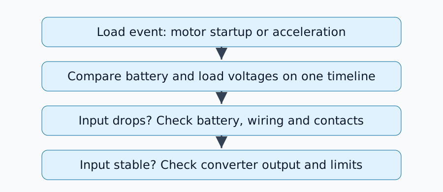
修复负载事件、电池充电、线路和设备版本。尽可能同时观察电池端子、转换器输入端、转换器输出端和计算机端子。平均值万用表显示可能会忽略短时压降。
使用示波器时,请验证探头额定值和接地情况,确保连接不会造成电路短路。不要探测无法确定接地的电路;选择合适的差分测量方法。测量时请始终在低压直流侧进行,切勿禁用保护电路。
根据观察结果选择下一步检查
| 观察结果 | 可能原因 | 下一步检查 |
|---|---|---|
| 电池电压下降 | 内阻、充电或电流限制 | 将匹配的负载条件与规格进行比较 |
| 电池稳定,转换器输入电压下降 | 线路或触点 | 各段电压下降 |
| 输入稳定,转换器输出电压下降 | 电流保护、瞬态响应或输入限制 | 数据手册和负载阶跃 |
| 转换器输出稳定,计算机输入电压下降 | 末端电缆或连接器 | 负载端子电压 |
此表缩小了假设范围;单个波形无法确定唯一原因。如果电源电压保持正常,请检查通信、复位信号、温度和软件。
电容器并非万能的解决方案
根据理想的放电关系 C=I\Delta t/\Delta V,在 0.2 V 的压降内提供 1 A 的额外电流持续 10 ms 需要 C=0.05 F,即 50,000 µF 的电容。这里假设电容器能够提供所有缺失的电流,但并不建议安装如此大的电容值。ESR、浪涌电流和转换器稳定性也至关重要。
添加元件之前,请检查共用线路电阻、触点和转换器的工作极限。您可以参考 TI 的电源管理文档 等资源,查找相关的元件数据手册和瞬态特性。
在相同条件下重复测试
记录修改情况、最小启动电压、复位次数、试验次数和电池状态。一次成功的运行并不能保证在所有充电状态和同时负载下都能成功。
每次试验使用一行记录,以避免成功启动掩盖间歇性复位。记录相同启动间隔内的最小电压;如果通道是在不同的试验中测量的,请将其标记为单独的测量值,而不是同时波形。
| 试验/更改 | 电池状态/同时负载 | 电池最小值 (V) | 转换器输入/输出最小值 (V) | 计算机最小值 (V) | 重置/观察 |
|---|---|---|---|---|---|
| 更改前/试验 1 | 记录条件 | 测量值 | 测量值 | 是/否;计时 | |
| 更改后/试验 1 | 匹配上述条件 | 测量值 | 测量值 | 测量值 | 是/否;计时 |
请将测量点、仪器设置和波形文件保存在表格旁边。电压限制应参考实际设备文档;这些空白条目仅为记录模板,并非实验结果。
评论
请先登录。
暂无数据。