Dead Reckoning Primer — Integrating Wheels, IMU, and GNSS to Track a Robot's Motion

The most primitive way for a robot to know that it "moved 1 m right, 2 m forward" is to keep adding up its own displacement. It integrates wheel rotation counts, motor speeds, and IMU angular rates over time to estimate its current position. This method is called dead reckoning. It keeps working even when GPS or a camera is temporarily unavailable, but small wheel slip or sensor bias turns into position error that grows over time.

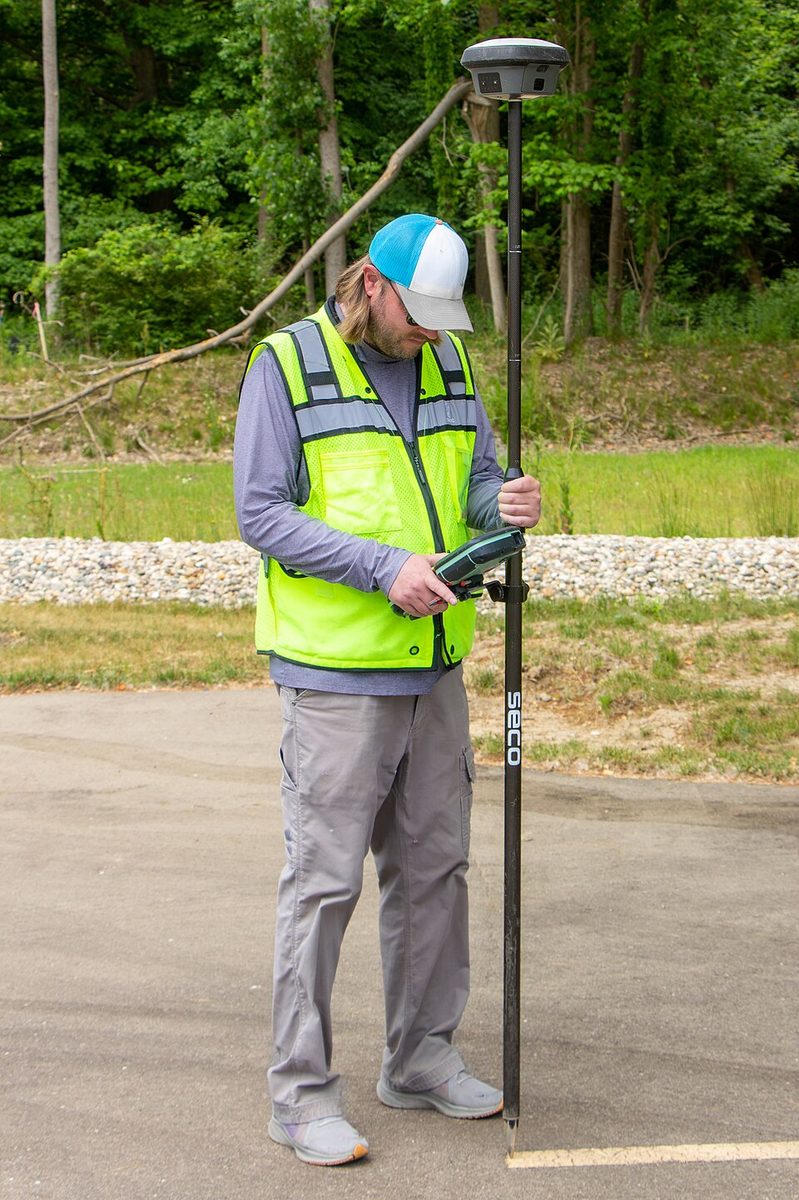Absolute GNSS observation

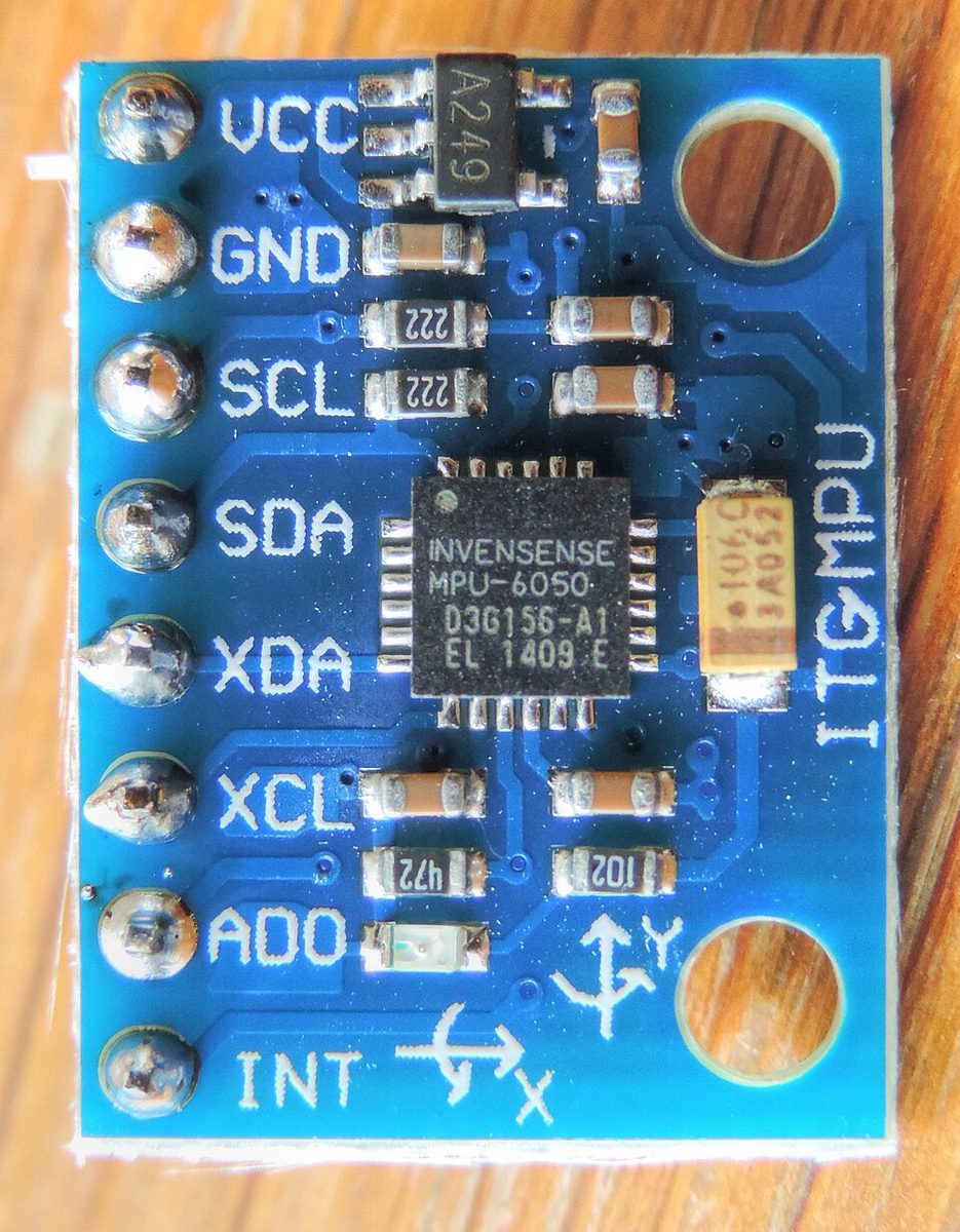Low-cost IMU example

Images: Surveyor Using GNSS Receiver with RTK Solution (SweetCanadianMullet, CC BY 4.0) / GY-521 MPU-6050 module (Nevit Dilmen, CC BY-SA 3.0), Wikimedia Commons. Representative sensors, not a mandatory hardware pairing.

30-Second Summary

• Dead reckoning predicts the current state from "the previous state plus the measured displacement." It can update at a high rate even without observations.
• In a differential-drive robot, the difference between the left and right wheels' displacement determines the turn angle, and their average determines the forward distance. Error in wheel radius and tread width shows up as a systematic curve.
• Odometry error accumulates through integration. Getting an absolute position requires correction from observations such as GNSS, LiDAR, camera, or reflective markers.
• An IMU is strong over short-term attitude changes, but position drifts rapidly when acceleration is double-integrated. Fusing wheels and an IMU via an EKF or a factor graph is the common approach.
• In implementation, timestamps, coordinate frames, left/right sign conventions, wheel radius, slip detection, and covariance must all be defined correctly from the start — get this wrong and even expensive sensors won't fix it.

1. Differential-Drive Kinematics

Let the left and right wheel radius be r, the distance between the wheels (tread) be b, and the left/right angular velocities be \omega_L,\omega_R. The wheels' linear velocities are v_L=r\omega_L and v_R=r\omega_R, so the vehicle center's translational velocity v and yaw rate \dot{\theta} are

Letting the pose at time k be (x_k,y_k,\theta_k) and the sampling period be \Delta t, simple Euler integration gives

When driving a constant-speed arc, using exact integration (the exponential map in body coordinates) keeps error small even at low speed and high turn rate.

Figure 1 — In differential drive, the difference between left and right speed creates yaw rate. Stopping one wheel lets the robot pivot around it.

2. Why Odometry Drifts

If wheel radius carries a 1% error and you assume left and right are the same while driving, you'll gradually turn even when you think you're going straight. Left/right encoder resolution, gear backlash, floor irregularities, tire wear, and load-induced deformation all become systematic error. If a wheel slips on a wet floor or gravel, the measured rotation and the actual displacement no longer match.

Attitude error \delta\theta produces lateral position error. For forward distance s, a short-time approximation gives

Drive 1 km with a 0.5-degree angle error, and the lateral offset reaches about 8.7 m. Simply expressing position error as "so many cm per second" can't capture the different error structures of driving straight, turning, and slipping.

Wheel odometry's covariance propagates the uncertainty of the left/right displacement into the pose and updates it accordingly. In implementation, covariance is inflated during turns or when slip is detected, so downstream sensor fusion doesn't over-trust the odometry.

3. Adding an IMU

Integrating the angular rate \omega_z from the IMU's gyroscope gives

where b_g is gyro bias and n_g is noise. Even at the instant a wheel slips, the short-term change in angular rate can still be measured, giving a smoother attitude estimate than wheels alone. When double-integrating acceleration to get velocity and position, error from bias b_a grows as

so an IMU alone cannot serve as a long-duration position sensor.

Combining wheels and an IMU: wheels handle low-frequency displacement, and the IMU handles high-frequency angular rate and acceleration. Roll/pitch are initialized from the gravity direction, and when a magnetometer or GNSS is available, an absolute yaw reference is added as well.

4. Correcting With an EKF or Factor Graph

One example state vector is

In the prediction step, a nonlinear motion model f is computed from wheels and IMU; when an observation arrives, the residual is used to correct it.

The Extended Kalman Filter (EKF) locally linearizes the nonlinear model via the Jacobian. GNSS position, LiDAR scan matching, camera feature points, and known-marker poses can all be brought in as observations \mathbf{z}. For large loops or revisits, past poses and observations are kept in a factor graph and the whole thing is re-optimized afterward.

For ROS 2 (assuming the Jazzy standard message definitions here), the wheel's nav_msgs/msg/Odometry, the IMU's sensor_msgs/msg/Imu, and the TF odom→base_link transform should use a common time basis. These message types correspond to the ROS 1 spellings nav_msgs/Odometry and sensor_msgs/Imu, but ROS 2 implementation details, QoS, and distro settings must be checked separately. robot_localization's EKF is a reasonable starting point for implementation, but zeroing out covariances or feeding in the same information twice makes the estimate unnaturally stiff.

5. How This Is Used in Current Robots

Indoor autonomous mobile robots (AMRs) constantly use wheel encoders and an IMU, resetting drift via LiDAR or camera map matching. In autonomous driving, wheel speed, steering angle, IMU, GNSS, and LiDAR are fused so the estimate holds up for seconds to tens of seconds even when GNSS drops out in a tunnel or under an elevated structure. In agricultural robots, mud, ruts, and slopes increase wheel slip, so RTK-GNSS, IMU, and implement force sensors are combined.

Underwater robots and spacecraft go long stretches without GNSS. A Doppler velocity log (DVL), star tracker, or terrain matching is added as a low-rate absolute observation to keep dead reckoning's covariance in check. What matters is passing the estimate to planning and control together with "how confident are we in this."

6. Implementation Checklist

1. Convert sensor timestamps to a common clock and measure latency.
2. Draw out the base_link, odom, and map coordinate frames and their right-handed sign conventions.
3. Identify wheel radius, tread, and encoder resolution through real driving tests.
4. Evaluate error separately for straight-line driving, steady turns, figure-eights, bumps, and low-friction surfaces.
5. Inflate covariance when slip or dropouts are detected, and correct when an absolute observation arrives.
6. Replay logs to confirm the same input produces the same estimate.

In testing, record not just endpoint position error but attitude error, maximum error, the 95th percentile, and the drift rate during dropouts. An estimate that's usually accurate but occasionally way off can't be used for safe path planning.

Summary

Dead reckoning is the foundational technique for estimating a robot's motion with the shortest possible delay. It integrates wheel displacement and IMU angular rate, suppressing drift with absolute observations from GNSS, LiDAR, or camera. Before adding more sensors, getting the motion model, timestamps, coordinate frames, and covariance right is what determines accuracy and repeatability.

References

• ROS 2 — tf2 documentation
• ROS 2 — robot_localization
• robot_localization — state estimation nodes and sensor parameters
• REP-105 — Coordinate Frames for Mobile Platforms
• ROS 2 Jazzy common_interfaces — standard message packages
• ROS 2 Jazzy sensor_msgs/Imu definition
• ROS 2 Jazzy nav_msgs/Odometry definition
• T. D. Barfoot, State Estimation for Robotics
• IEEE Robotics and Automation Society